DEVELOPING RECOMMENDATIONS FOR UNDERTAKING CPUE
STANDARDISATION USING OBSERVER PROGRAM DATA
Lilis Sadiyah1), Natalie Dowling2) and Budi Iskandar Prisantoso1) 1) Research Centre for Fisheries Management and Conservation-Jakarta
2) CSIRO Marine and Atmospheric Research-Tasmania Australia
Received January 3-2012; Received in revised form June 8-2012; Accepted June 12-2012
email: [email protected]
ABSTRACT
Abundance indices based on nominal CPUE do not take into account confounding factors such as fishing strategy and environmental conditions, that can decouple any underlying abundance signal in the catch rate. As such, the assumption that CPUE is proportional to abundance is frequently violated. CPUE standardisation is one of the common analyses applied. The aims of this paper were to provide a statistical modelling framework for conducting CPUE standardisations using the Observer Program data for bigeye tuna, yellowfin tuna, albacore and southern bluefin tuna, and provide a comparison in the trends between the nominal CPUEs and their standardised indices obtained. The CPUE standardisations were conducted on the Observer Program collected between 2005 and 2007, by applying GLM analysis using the Tweedie distribution. The results suggested that year, area, HBF and bait factors significantly influenced the nominal CPUEs for the four tuna species of interest. Some extreme peaks and troughs in the nominal time series were smoothed in the standardised CPUE time series. The high degree of temporal variability that is still shown in the standardised CPUE trends suggests that the data are too sparse to give any meaningful indication of proxy abundance. Nevertheless, this may also suggest that variables used in the GLMs do not sufficiently account for all of the confounding factors, or abundance may indeed be truly variable.
KEYWORDS: CPUE standardisation, observer program, tweedie distribution, Indian Ocean
INTRODUCTION
It is essential to understand temporal trends in its abundance in order to manage a fish population effectively (Ortega-Garcia et al., 2003, Chen et al., 2004, Maunder et al., 2006a). For commercial longline vessels, CPUE data are the main source of abundance information (Maunder & Punt, 2004, Maunder et al., 2006b, Ward & Hindmarsh, 2007, Bigelow et al., 1999) as fishery-independent data are impractical to collect (Bishop, 2006, Maunder et al., 2006b). Abundance indices based on nominal CPUE do not take into account confounding factors such as fishing strategy (Bach et al., 2000) (including fishing power & catchability (Ward, 2008)), and environmental conditions, that can decouple any underlying abundance signal in the catch rate (Polacheck, 1991, Hinton & Nakano, 1996, Hampton et al., 1998). As such, the assumption that CPUE is proportional to abundance is frequently violated (Maunder et al.,
2006b) and, in turn, the relative abundance indices based on nominal CPUE data can be misleading (Maunder & Punt, 2004) or even problematic (Beverton & Holt, 1957, Hilborn & Walters, 1991, Walters, 2003, Ortega-Garcia et al., 2003). Thus, effects of those confounding factors need to be statistically filtered out in order to be able to use the time series of CPUE as a proxy of relative abundance with any accuracy
Accordingly, CPUE standardisation is one of the most common analyses applied to yield a proxy index of fish abundance (Maunder & Punt, 2004, Bigelow & Maunder, 2007, Maunder et al., 2006b). Several methods have been developed (e.g. Gulland, 1956, Beverton & Holt, 1957, Robson, 1966, Honma, 1974) to standardise CPUE, including generalised linear modelling (GLM), generalised additive modelling (GAM), generalised linear mixed modelling (GLMM) and the delta approach1; however, GLM is the
predominant approach (Dowling & Campbell, 2001, Maunder et al., 2006a, Maunder and Punt, 2004, Su
et al., 2008), having been applied in many fisheries (Venables & Dichmont, 2004) to standardise CPUE data (e.g. Goñi et al., 1999, Tascheri etal., 2010). Su
et al. (2008) applied GLM, GAM and a delta approach to standardise BET CPUE on Taiwanese distant-water longline fishery, and suggested that any of the three methods individually is sufficiently flexible to capture the key features of the data.
catch rates and understanding the process behind the trends (Minami et al., 2007). CPUE standardisation using statistical distributions that allow for zero observations has been applied in some cases (e.g. Candy, 2004, Basson & Farley, 2005) by fitting GLM using Tweedie family distributions. The Tweedie distribution can deal with zero values and can sensibly incorporate zero catch data with non-zero catch data into a single model (Candy, 2004). In addition, the Tweedie distribution can accommodate larger ranges of models for count data than the Poisson, Negative Binomial, Zero-inflated Poisson and Zero-inflated Negative Binomial models (Minami et al., 2007). The Tweedie distribution approach was therefore adopted within this paper.
The aims of this paper were to provide a statistical modelling framework for conducting CPUE standardisations using the Observer Program data for bigeye tuna, Thunnus obesus (BET), yellowfin tuna,
T. albacares (YFT), albacore, T. alalunga (ALB) and southern bluefin tuna, T. maccoyii (SBT), and provide a comparison in the trends between the nominal CPUEs and their standardised indices obtained. Since the Observer Program data set is only a short time series, meaningful temporal trends are not anticipated. However, the exercise of standardisation is valid both in terms of providing a template for undertaking standardisations as long-term Observer Program data become available over time as the Observer Program evolves.
This paper attempts to develop recommendations for ongoing monitoring and analysis, and providing a statistical modelling framework to undertake CPUE standardisations for future data.
METHODS
The standardisation should incorporate all of the extraneous variables influencing CPUE in order to take into account their impacts. The effect of these variables is then eliminated and a standardised value reconstructed that is hoped to be directly proportional to abundance. Obviously the extent to which this can occur is limited by the amount of available data. The CPUE standardisations in this paper were conducted by applying GLM analysis using the Tweedie distribution. For each tuna species, standardised CPUEs were then plotted together with the nominal CPUE. This enabled comparison of the nominal and standardised CPUEs.
Data Overview
A total of 793 set-by-set data span from August 2005 to December 2007 were obtained from Indonesia’s Indian Ocean trial Observer Program on tuna longline vessels based at Benoa Fishing Port. 41 records were excluded due to incomplete information on fishing techniques and environmental data. The Observer Program data consist of catch and effort data, information on fishing practices, and environmental data (summarised below).
Catch and effort data
Catch and effort data were recorded as the number of fish and the number of hooks recorded per set, respectively. The catch for this fishery consists of four tuna species, BET, YFT, ALB and SBT, and other byproduct species. The analyses in this chapter are only concerned with the four tuna species. Species-specific catch (number of fish) was used as the response variable and the log of effort (number of hooks) was assigned as an offset in the GLM analyses.
Fishing practices
Factors considered under the category of targeting strategies include the number of hooks between floats (HBF), the bait species/combination used, the area fished, the start time of the set, and gear characteristics. However, different fishing practices were sometimes used by vessels to target the same species (pers comm. with the observers, 2007). These different practices may result in dissimilar catchabilities that will confound the nominal CPUE trend (Maunder & Punt, 2004). Thus, incorporating these fishing practices into the GLM analysis is imperative. The following information on fishing strategies was recorded and included in GLM analyses:
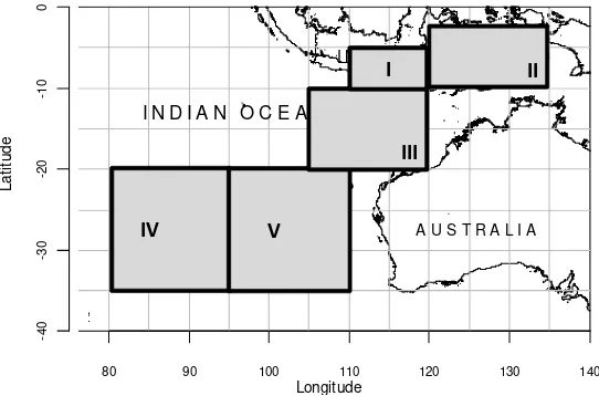
a. Fishing area
b. HBF or number of branch lines
HBF information was available for each recorded set, and varied from 4–21 HBF. The HBF information was incorporated as a categorical covariate in the GLM. It was assigned as 1 if HBF <10 hooks (surface longline), and 2 if HBF e”10 hooks (deep longline) (Table 1).
c. Bait combination
There are six main bait species used as follows: Lemuru, Sardinella spp. (LMR); Milkfish, Chanos chanos (MIL); Scad mackerel, Decapterus spp. (RUS); Gizzard shad, Anodontostoma chacunda
(CHG); Frigate Tuna, Auxis spp. (FRI); and Squid,
Loligo spp.(CMI). However, the fishers sometimes deployed a combination of these bait species within one catenary (between two floats). There were 22 bait combinations recorded and each bait combination was assigned to a unique bait type index. The 22 bait types were included as a categorical variable in the GLM (Table 1).
d. Vessel identification (Vessel Id)
A Vessel identification factor embraces all attributes of a vessel, such as size, capacity and electronic equipment, and its crew that determine the success of the vessel’s fishing activity, such as the ability of the crew to find good fishing grounds and to use the gear efficiently (Campbell & Hobday, 2003). It is worthwhile taking into account the effect of each individual vessel on catch rates. The Vessel Identification factor included in the GLM as a categorical variable (Table 1).
e. Start time of set
The time at which the set commenced was employed to represent fishing time and was taken into account as a categorical variable in the GLM and assigned into 6 levels (Table 1). This assignment of the start time of set was adopted from Campbell & Hobday (2003).
L
a
ti
tu
d
e
80 90 100 110 120 130 140
-4
0
-3
0
-2
0
-1
0
0
Longitude
I N D I A N O C E A N
A U S T R A L I A I N D O N E S I A
IV V
III
I II
Figure 1. Fishing positions recorded by the observers (dot) and the five area categories used in the CPUE standardisation (shaded area)
f. Lengths of float line, branch line and main line
In addition to the HBF, the actual fishing depth of the longline is influenced by the lengths of the float line and branch line (Bigelow et al., 2002), and by the length of main line between floats (Suzuki et al., 1977). However, for the Benoa-based longline vessels this latter gear change is impractical to undertake within one trip (pers comm. with the observers, 2007). To eliminate effects of these gear configurations on the nominal CPUEs, these three variables are included as continuous covariates in the GLM analysis (Table 1).
g. Age of main line
Environmental data
Types of environmental data included in the CPUE standardisation are as follows:
a. Phase of the moon
Moon phase information is available as a daily index of moon fraction for all recorded sets and ranges between 0 and 1 (from new moon to full moon). The moon phase was incorporated in the CPUE standardisation as a continuous variable in the GLM analysis. To account for the effect of cyclic behaviour, the moon phase was incorporated as a new variable called “MOON” in the GLM analysis (Table 1), which is defined by the following function (equation 1):
MOON =sin (2 x moon phase) + cos (2 x moon phase) ...1)
where 2 translates the variable into radians and moon phase ranges between 0 and 1.
b. Sea surface temperature (SST)
Sea surface temperature information was calculated using the Spatial Dynamics Ocean Data Explorer (SDODE) in Matlab and was available for each set. To account for a possible non-linear (quadratic) relationship between CPUE and SST, the SST was assigned as a quadratic variable (expressed in R as poly (SST, 2)) and incorporated as a continuous variable in the GLM analysis (Table 1).
c. Sea Conditions
Sea conditions were incorporated using the Beaufort scale (created by Sir Francis Beaufort in 1805) as a continuous variable in the GLM analysis (Table 1).
∏ ∏
∏
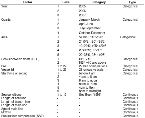
Factor Level Category Type
Year 1 2005 Categorical
2 2006
3 2007
Quarter 1 January-March Categorical
2 April-June
3 July-September
4 October-December
Area 1 5°-10°S; 110°-120°E Categorical
2 2°-10°S; 120°-135°E
3 10°-20°S; 105°-120°E
4 20°-35°S; 80°-95°E
5 20°-35°S; 95°-110°E
Hooks between floats (HBF) 1 HBF <10 Categorical
2 HBF =10 and above
Bait 1 to 22 22 bait combinations Categorical
Vessel Id 1 to 23 23 unique vessels Categorical
Start time of setting 1 before 4 am Categorical
2 4 am to 8 am
3 8 am to noon
4 noon to 4pm
5 4pm to 8pm
6 8pm to midnight
Sea conditions 1 to 12 See Beer (1996) Continuous
Length of float line - - Continuous
Length of branch line - - Continuous
Length of main line - - Continuous
Age of main line - - Continuous
MOON - - Continuous
Sea surface temperature (SST) - - Continuous
Generalised linear model
The exploratory variables described previously are summarisedinTable 1. The first seven variables were fitted as categorical (factor) variables while variables 8-14 were fitted as continuous (numerical) variables in the GLM model (equation 2).
The catch by each level of each categorical variable was examined to determine level/s of each categorical variable that only have zero catches for the species of interest. These level/s were excluded as being uninformative prior to the GLM analyses for that species (e.g. if there are only zero catches for the species of interest using a certain bait type, then that bait type is excluded).
CPUE was defined as the catch, in numbers of fish, per 100 hooks of effort. Since the CPUE is a ratio of two random variables, modelling the distribution of CPUE can be complicated (Candy, 2004). Therefore, catch data and the log of effort were used as the response variable and an offset in the GLM model, respectively, and a log-link function was used (Candy, 2004, Basson & Farley, 2005). The catch data was modelled using the Tweedie distribution or the compound Poisson-Gamma distribution (see Jørgensen (1997) & Candy (2004) for a full explanation of the Tweedie distribution). Subsequently, the catch was modelled using all variables mentioned above as follows (equation 2), referred to as the “full model”, hereafter:
where c is a constant (intercept), i corresponds to the ithdata record, n is the coefficient for the nth variable and e is the error term (normally distributed). Each categorical variable has a separate coefficient value for each level of the variable, with j corresponding to the jth coefficient value for the associated level of the categorical variable.
The Tweedie distribution has a power variance function, with the power parameter (k) (Candy, 2004, Basson & Farley, 2005). Values of k for the Tweedie distributions range between 1 and 2, which is appropriate for zero catch observations (Basson & Farley, 2005). k equals to 0, 1 and 2 associated with normal, Poisson and gamma distributions respectively
(Candy, 2004, Basson & Farley, 2005). The first step of the GLM process was to select the value of k (1 < k < 2) using the randomised quantile residual diagnostic. This was done by running the full model (equation 2) for a range of k values between 1 and 2. The value of k with the flattest plot in the Scale-location of the quantile residuals, and the most normally distributed quantile residuals in the normal QQ plot and the histogram of residuals, was chosen. To enable the use of the Tweedie distributions within the GLM framework and to produce the quantile residual diagnostic plots, respectively, the “Tweedie” and “Statmod” functions in R were used.
Once the k-value had been determined, the selection of the best model/s was done using the stepwise AIC (Akaike Information Criterion) in R using the “MASS” package. The best model was the one with the lowest AIC value. Models that are within 5 AIC units of the best model, while yielding qualitatively similar CPUE trends, are also included in a short-list of “best options” (pers comm. with Mark Bravington, Natalie Kelly and Marinelle Basson). A summary table of GLM results for the best and full model is provided, but it should be emphasised that the model selection was done using the stepwise AIC, not the statistics in the summary table, as stepwise AIC is preferable to ANOVA significance to determine the optimal model/ s (pers comm. with Mark Bravington, Natalie Kelly & Marinelle Basson). For the best model, the diagnostic plots were again checked to confirm that no counter-intuitive trend were present. These diagnostic plots are presented in Appendix 1.
Interaction terms between year and area, and between quarter and area were trialled to be incorporated in the GLM analysis. However, as a result of a lack of data across all possible quarter-area combinations, the coefficients of the interaction terms were infinite and this resulted in null value of the indices. Therefore, these interaction terms were not included in the final GLM.
The abundance indices for each of the four tuna species were estimated by reconstructing a standardised CPUE value using the “predict” function in R (“Stats” package) on a revised dataset, where those exploratory variables not equal to Year and Quarter were set constant. The constant values chosen for the confounding factors were typically the median value of each of the variables. Nominal CPUEs and standardised indices were normalised relative to their respective grand means in order to yield directly comparable relative values.
RESULTS
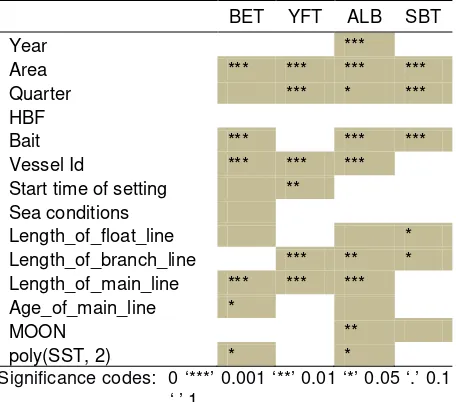
The “best model options” for BET, YFT, ALB and SBT as determined according to the stepwise AIC criterion are presented in Table 2-Table 5. The best model – that has the smallest AIC, for each species -was used to predict the standardised CPUEs (Figure 2). The randomised quantile residual diagnostic for the best model is given in Appendix 1. The results of analyses of variance for the best (for BET, YFT and SBT) models are given in Appendix 2.The results of the best model for each data set are summarised in Table 6. Shaded cells indicate the variables included in the best model for each species.
The nominal CPUE trend for the four tuna species was significantly influenced by different factors associated with fishing practices and/or environmental
conditions. For BET, the Area, Bait, Vessel Id, and length of main line covariates were highly significant (p-value <0.1%), followed by the age of the main line and SST (p-value<5%). Area, Quarter, Vessel Id, length of branch line and length of main line were highly significant (p-value <0.1%) for the YFT GLM, followed by the start time of set covariate (p-value<1%). For ALB GLM, Year, Area, Bait, Vessel Id and length of main line were highly significant (p-value <0.1%) followed by length of branch line and MOON (p-value <1%), and then Quarter and SST (p-value <5%). Area, Quarter and Bait had a strongly significant influence on the nominal CPUE for SBT (p-value <0.1%), followed by length of float line and length of branch line (p-value <5%). Area, Quarter, Bait, Vessel Id and length of main line covariates are the most common variables that significantly influenced the nominal CPUEs of the four tuna species in GLMs.
Table 2. List of model option for BET in order of increasing AIC (such that Model 1 is the statistically optimal model). Model option no. 4 is used as an alternative model (with the inclusion of Year factor).
No. Model Options AIC
1. Catch ~ Area + Quarter + Bait + Vessel_Id + Start_time_of_setting +
sea_conditions + Length_of_float_line + Length_of_main_line + Age_of_main_line + poly(SST, 2) + offset(log(TotalHook))
3124.26
2. Model 1 + Length_of_branch_line 3125.96
3. Model 1 + Length_of_branch_line + MOON 3127.72
4. Model 1 + Year + Length_of_branch_line + MOON 3129.17
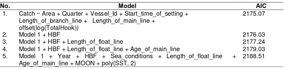
No. Model AIC
1. Catch ~ Area + Quarter + Vessel_Id + Start_time_of_setting +
Length_of_branch_line + Length_of_main_line + offset(log(TotalHook))
2175.07
2. Model 1 + HBF 2176.03
3. Model 1 + HBF + Length_of_float_line 2177.24
4. Model 1 + HBF + Length_of_float_line + Age_of_main_line 2179.03
5. Model 1 + Year + HBF + Sea_conditions + Length_of_float_line +
Age_of_main_line + MOON + poly(SST, 2)
2188.51
Table 3. List of model option for YFT in order of increasing AIC (such that Model 1 is the statistically optimal model). Model option no. 5 is used as an alternative model (with the inclusion of Year factor).
No. Model AIC
1. Catch ~ Year + Area + Quarter + Bait + Vessel_Id + Length_of_float_line
+ Length_of_branch_line + Length_of_main_line + Age_of_main_line + MOON + poly(SST, 2) + offset(log(TotalHook))
2266.21
2. Model 1 without Age_of_main_line 2266.23
3. Model 1 + HBF 2267.31
4. Model 1 + HBF + Sea_conditions 2269.23
No. Model AIC
1. Catch ~ Area + Quarter + Bait + Length_of_float_line + Length_of_branch_line + MOON + offset(log(TotalHook))
796.81
2. Model 1 + Length_of_main_line 797.6 3. Model 1 + Length_of_main_line + Age_of_main_line 799.32 4. Model 1 + HBF + Length_of_main_line + Age_of_main_line 801.15 5. Model 1 + Year + HBF + Vessel_Id + Start_time_of_setting + Sea_conditions +
Length_of_main_line + Age_of_main_line
820.84 Table 5. List of model option for SBT in order of increasing AIC (such that Model 1 is the statistically optimal
model). Model option no. 5 is used as an alternative model (with the inclusion of Year factor).
Table 6. Summary of significance level for each explanatory variable in the GLMs fitted using the data set for each species.
BET YFT ALB SBT
Year ***
Area *** *** *** ***
Quarter *** * ***
HBF
Bait *** *** ***
Vessel Id *** *** ***
Start time of setting **
Sea conditions
Length_of_float_line *
Length_of_branch_line *** ** *
Length_of_main_line *** *** ***
Age_of_main_line *
MOON **
poly(SST, 2) * *
Significance codes: 0 ‘***’ 0.001 ‘**’ 0.01 ‘*’ 0.05 ‘.’ 0.1 ‘ ’ 1
Variable included in the best GLM model (i.e. the smallest AIC)
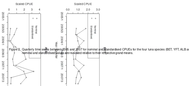
Quarterly nominal and standardised CPUEs (relative abundance indices) between 2005 and 2007 are shown in Figure 2, and the predicted values of the standardised CPUEs and the associated standard errors are given in Table 7. The standardised CPUEs were predicted using the best models for each species (Table 2-Table 5). The nominal and standardised values are re-scaled relative to their respective grand means. Since only a short time series was available, it is difficult to infer any strong temporal or seasonal abundance patterns, but this approach forms a template for undertaking standardisations as a longer time series of data becomes available.
The best models for BET, YFT and SBT (Table 2, Table 3 and Table 5) do not include the Year factor. The next best models that have the lowest AIC while including the Year effect and have the smallest AIC (termed “alternative models” were plotted for those species (not presented in this paper). The standardised CPUEs for 2007 were slightly higher for BET and YFT, and more than double for SBT in any quarters relative to those in 2006. However, the comparison within this chapter used the best model for all species.
Comparing the standardised CPUE trends between species for the GLMs, the standardised time series was relatively stable for BET, YFT and SBT, except for the two spikes for BET, YFT and SBT (in the first quarter of 2006 and 2007) (Figure 2). The ALB standardised time series was variable but consistently higher in quarter 3 of 2006 and 2007. This pattern in the standardised indices had previously been obscured by the fishing practices, most significantly by fishing area, bait, vessel, length of main line and length of branch line (in order of decreasing statistical significance) (Table6).
0.0 1.0 2.0 3.0
Figure 2. Quarterly time series between 2005 and 2007 for nominal and standardised CPUEs for the four tuna species (BET, YFT, ALB and SBT). The nominal and standardised values are re-scaled relative to their respective grand means.
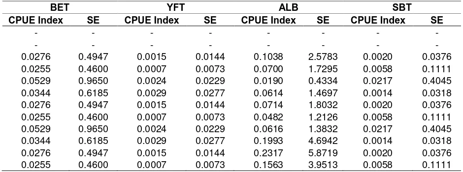
Table 7. Predicted values of standardised CPUEs for BET, YFT, ALB and SBT with its associated standard errors. These standardised CPUEs are from very scarce data, thus they are not for use in any stock assessments.
BET YFT ALB SBT
CPUE Index SE CPUE Index SE CPUE Index SE CPUE Index SE
- - - -
- - - -
0.0276 0.4947 0.0015 0.0144 0.1038 2.5783 0.0020 0.0376
0.0255 0.4600 0.0007 0.0073 0.0700 1.7295 0.0058 0.1111
0.0529 0.9650 0.0024 0.0229 0.0190 0.4334 0.0217 0.4045
0.0344 0.6185 0.0029 0.0277 0.0614 1.4697 0.0014 0.0318
0.0276 0.4947 0.0015 0.0144 0.0714 1.8032 0.0020 0.0376
0.0255 0.4600 0.0007 0.0073 0.0482 1.2126 0.0058 0.1111
0.0529 0.9650 0.0024 0.0229 0.0616 1.3832 0.0217 0.4045
0.0344 0.6185 0.0029 0.0277 0.1993 4.6942 0.0014 0.0318
0.0276 0.4947 0.0015 0.0144 0.2317 5.8719 0.0020 0.0376
0.0255 0.4600 0.0007 0.0073 0.1563 3.9513 0.0058 0.1111
DISCUSSION
Across the four tuna species, temporal trends of nominal CPUEs were significantly influenced by different factors either associated with fishing practices and/or environmental conditions. Area, Quarter, Bait, Vessel Id and length of main line covariates were the most common variables that significantly influenced the nominal CPUEs of the four tuna species. Similarly, effects of area and season (month or quarter) were reported to significantly influence nominal CPUEs of YFT caught by Japanese longline vessels (from 1975-1998) (Nishida, 2000) and Japanese, Korean and Taiwanese longline vessels (from 1970-1992) (Nishida, 1995) operating in the Western Indian Ocean. Importantly, by eliminating the effect of fishing strategies and environmental variables from the CPUE signal, some extreme peaks and troughs in the nominal CPUE time series were smoothed in the standardised CPUE time series. The high degree of temporal variability that is still shown in the standardised CPUE trends further suggests that the data are too sparse give an accurate indication of abundance. However, this may also suggest that variables used in the GLMs do not sufficiently account for all of the confounding factors, or the abundance may indeed be truly variable.
In this current standardisation, several models including interaction terms between year and area, between quarter and area, and between year and quarter were trialled. However, coefficients of the interaction terms were infinite and this resulted in null indices. This again was due to the data scarcity when
it was grouped in combination of the two effects (i.e. year and area, quarter and area, and year and quarter). Therefore, these interaction terms were removed from the GLM. As more data become available in future, it will be more feasible to include interaction terms in the GLMs. Such interactions are likely to be significant, given the experience of other researchers working with larger data sets. Maunder & Punt, (2004) stated that interactions among factors commonly occur when standardising catch and effort data (e.g. Okamoto & Miyabe, 1998, Matsumoto, 2000, Nishida, 2000, Okamoto & Shono, 2008), meaning that simple interpretations of the main effect cannot be used as the basis to develop an index of abundance (Maunder & Punt, 2004).
CONCLUSION
It was suggested that year, area, HBF and bait factors significantly influenced the nominal CPUEs for the four tuna species of interest. By eliminating the effect of fishing strategies and environmental variables from the nominal CPUE trend, some extreme peaks and troughs in the nominal time series were smoothed in the standardised CPUE time series. The high degree of temporal variability that is still shown in the standardised CPUE trends suggests that the data are too sparse to give any meaningful indication of proxy abundance. Nevertheless, this may also suggest that variables used in the GLMs do not sufficiently account for all of the confounding factors, or abundance may indeed be truly variable.
ACKNOWLEDGEMENTS
The authors wish to thank Indonesia’s tuna fishing companies and the Bali Office of WASKI for their cooperation, assistance and support for the trial observer program. We also would like to thank ACIAR and RCCF for their funding through research collaboration in the project FIS/2002/074: Capacity development to monitor, analyse and report on Indonesian tuna fisheries. In addition, we would like to thank Dr. Marinelle Basson, Dr. Mark Bravington and Dr. Natalie Kelly for their assistance in applying the Generalised Linear Model with Tweedie distribution and its interpretation. Last but not least, the Observer team, without whom this research would not have been possible, we are extremely grateful.
REFERENCES
Bach, P., Dagorn, L. & Misselis, C. 2000. The role of bait type on pelagic longline efficiency. ICES Annual Science Conference Theme Session J: Efficiency, selectivity and impacts of passive gears, Brugge, Belgium, CM 2000/J:01.
Basson, M. & Farley, J. 2005. Commercial spotting in the Australian surface fishery, updated to include the 2004/5 fishing season. CCSBT 6th Meeting of the Stock Assessment Group and 10th Meeting of the Extended Scientific Committee, Taipe, Taiwan, 29 August - 3 September, and 5-8 September 2005. CCSBT-ESC/0509/23.
Beer, T. 1996. Environmental Oceanography, Boca Raton, CRC Press.
Beverton, R. J. H. & Holt, S. J. 1957. On the dynamics of exploited fish populations. Fishery Investigations. 19: 533 pp.
Bigelow, K. A., Boggs, C. H. & He, X. 1999. Environmental effects on swordfish and blue shark catch rates in the US North Pacific longline fishery.
Fisheries Oceanography. 8: 178-198.
Bigelow, K. A., Hampton, J. & Miyabe, N. 2002. Application of a habitat-based model to estimate effective longline fishing effort and relative abundance of Pacific bigeye tuna (Thunnus obesus). Fisheries Oceanography. 11: 143-155.
Bigelow, K. A. and Maunder, M. N. (2007) Does habitat or depth influence catch rates of pelagic species?
Canadian Journal of Fisheries and Aquatic Sciences. 64: 1581-1594.
Bishop, J. 2006. Standardizing fishery-dependent catch and effort data in complex fisheries with technology change. Reviews in Fish Biology and Fisheries. 16: 21-38.
Bjordal, A. & Lokkeborg, S. 1996. Longlining, London, Fishing News Books. 156 pp.
Campbell, R. A. & Hobday, A. J. 2003. Swordfish-environment-seamount-fishery interactions off eastern Australia. Report to the Australian Fisheries Management Authority. Hobart, CSIRO Marine Research. 1876996471. 97 pp.
Candy, S. G. 2004. Modelling catch and effort data using generalised linear models, the Tweedie distribution, random vessel effects and random stratum-by-year effects. CCAMLR Science. 11: 59-80.
Chen, J., Thompson, M. E. & Wu, C. 2004. Estimation of fish abundance indices based on scientific research trawl surveys. Biometrics. 60: 116-123.
Dowling, N. & Campbell, R. 2001. Assessment of the Japanese longline fishery off Western Australia: 1980-1996. 1st meeting of the Stock Assessment Group for the Southern and Western Tuna and Billfish Fishery, Fremantle, Western Australia, 26-28 February 2001.
Goñi, R., Alvarez, F. & Adlerstein, S. 1999. Application of generalized linear modeling to catch rate analysis of Western Mediterranean fisheries: the Castellón trawl fleet as a case study. Fisheries Research. 42: 291-302.
Gulland, J. A. 1956. On the fishing effort in English demersal trawl fisheries. Fishery Investigations.
Hampton, J., Bigelow, K. & Labelle, M. 1998. A summary of current information on the biology, fisheries and stock assessment of bigeye tuna (Thunnus obesus) in the Pacific Ocean, with recommendations for data requirements and future research. Oceanic Fisheries Programme Technical Report No. 36. Noumea, New Caledonia, Secretariat of the Pacific Community. p 1-46.
Hilborn, R. & Walters, C. J. 1991. Quantitative fisheries stock assessment : choice, dynamics, and uncertainty, New York, Chapman and Hall. 580pp.
Hinton, M. G. & Nakano, H. 1996. Standardizing catch and effort statistics using physiological, ecological, or behavioral constraints and environmental data, with an application to blue marlin (Makaira nigricans) catch and effort data from Japanese longline fisheries in the Pacific. Inter-American Tropical Tuna Commission Bulletin. 21: 171-200.
Honma, M. 1974. Estimation of overall effective fishing intensity of tuna longline fishery - yellowfin tuna in the Atlantic Ocean as an example of seasonally fluctuating stocks. Bull. Far Seas Fish. Res. Lab.
10: 63-86.
Jørgensen, B. 1997. Theory of Dispersion Models,
London, Chapman and Hall.
Matsumoto, T. 2000. Standardized CPUE for bigeye caught by the Japanese longline fishery in the Indian Ocean, 1952-1999. Second Session of the IOTC Working Party on Tropical Tunas, Victoria, Seychelles 23-27 September 2000. IOTC-2000-WPTT-08.
Maunder, M. N., Hinton, M. G., Bigelow, K. A. & Langley, A. D. 2006a. Developing indices of abundance using habitat data in a statistical framework. Bulletin of Marine Science. 79: 545-559.
Maunder, M. N. & Punt, A. E. 2004. Standardizing catch and effort data: a review of recent approaches. Fisheries Research. 70: 141-159.
Maunder, M. N., Sibert, J. R., Fonteneau, A., Hampton, J., Kleiber, P. & Harley, S. J. 2006b. Interpreting catch per unit effort data to assess the status of individual stocks and communities. ICES J. Mar. Sci. 63: 1373-1385.
Minami, M., Lennert-Cody, C. E., Gao, W. & Román-Verdesoto, M. 2007: Modeling shark bycatch: The zero-inflated negative binomial regression model with smoothing. Fisheries Research. 84: 210-221.
Nishida, T. 1995. Preliminary resource assessment of yellowfin tuna (Thunnus albacares) in the Western Indian Ocean by the stock-fishery dynamic model. Sixth Expert Consultation on Indian Ocean Tunas, Colombo, Sri Lanka, 25-29 September 1995. IPTP/95/EC602-13.
Nishida, T. 2000. Standardization of the Japanese longline catch rates of adult yellowfin tuna (Thunnus albacares) in the Western Indian Ocean by general linear model (1975-98). Second Session of the IOTC Working Party on Tropical Tunas, Victoria, Seychelles 23-27 September 2000. IOTC-2000-WPTT-10.
Okamoto, H. & Miyabe, N. 1998. Updated standardized CPUE of bigeye caught by the Japanese longline fishery in the Indian Ocean.
Seventh Expert Consultation on Indian Ocean Tunas, Victoria, Seychelles, 9-14 November 1998. IPTP/98/EC7-25.
Okamoto, H. & Shono, H. 2008. Standardization of annual and quarterly CPUE for yellowfin tuna caught by Japanese longline fishery in the Indian Ocean up to 2007 using general linear model.
Tenth Session of the IOTC Working Party on Tropical Tunas, Bangkok, Thailand, 23-31 October 2008. IOTC-2008-WPTT-19.
Ortega-Garcia, S., Lluch-Belda, D. & Fuentes, P. A. 2003. Spatial, seasonal, and annual fluctuations in relative abundance of yellowfin tuna in the eastern Pacific Ocean during 1984-1990 based on fishery CPUE analysis. Bulletin of Marine Science.
72: 613-628.
Polacheck, T. 1991. Measures of effort in tuna longline fisheries: changes at the operational level.
Fisheries Research. 12: 75-87.
Robson, D. S. 1966. Estimation of the relative fishing power of individual ships. International Commission Northwest Atlantic Fisheries Research Bulletin. 3: 5-14.
Su, N. J., Yeh, S. Z., Sun, C. L., Punt, A. E., Chen, Y. & Wang, S. P. 2008. Standardizing catch and effort data of the Taiwanese distant-water longline fishery in the Western and Central Pacific Ocean for bigeye tuna, Thunnus obesus. Fisheries Research. 90: 235-246.
Suzuki, Z., Warashina, Y. & Kishida, M. 1977. The comparison of catches by regular and deep tuna longline gears in the Western and Central Equatorial Pacific. Bull. Far Seas Fish. Res. Lab.
15: 51-89.
Tascheri, R., Saavedra-Nievas, J. C. & Roa-Ureta, R. 2010. Statistical models to standardize catch rates in the multi-species trawl fishery for Patagonian grenadier (Macruronus magellanicus) off Southern Chile. Fisheries Research, 105: 200-214.
Venables, W. N. & Dichmont, C. M. 2004. GLMs, GAMs and GLMMs: an overview of theory for applications in fisheries research. Fisheries Research. 70: 319-337.
Walters, C. 2003. Folly and fantasy in the analysis of spatial catch rate data. Canadian Journal of Fisheries and Aquatic Sciences. 60: 1433-1436.
Ward, P. 2008. Empirical estimates of historical variations in the catchability and fishing power of pelagic longline fishing gear. Reviews in Fish Biology and Fisheries. 18: 409-426.
Appendix 1. Randomised quantile residual diagnostic for BET, YFT, ALB and SBT GLMs
a. BET c. ALB
Appendix 2. Analysis of variance for BET, YFT, ALB and SBT GLMs using the best models.
1. BET indices
Df Deviance Resid. Df Resid. Dev F Pr(>F)
NULL 789 2652.82
Area 4 708.46 785 1944.36 91.5532
< 2.2e-16 ***
Quarter 3 0.26 782 1944.1 0.0455 9.87E-01
Bait 18 292.71 764 1651.39 8.4059
< 2.2e-16 ***
Vessel Id 22 194.59 742 1456.8 4.5721 3.88E-11 ***
Start time of setting 5 16.74 737 1440.06 1.7302 1.25E-01
Sea conditions 1 1.82 736 1438.24 0.9425 3.32E-01
Length_of_float_line 1 0.12 735 1438.12 0.0612 0.80465
Length_of_main_line 1 38.38 734 1399.74 19.8385 9.75E-06 ***
Age_of_main_line 1 9.04 733 1390.7 4.6744 0.03094 *
poly(SST, 2) 2 17.55 731 1373.14 4.5372 0.01101 *
Significance codes: 0 ‘***’ 0.001 ‘**’ 0.01 ‘*’ 0.05 ‘.’ 0.1 ‘ ’ 1
2. YFT indices
Df Deviance Resid. Df Resid. Dev F Pr(>F)
NULL 742 2543.28
Area 4 326.54 738 2216.74 37.986 < 2.2e-16 ***
Quarter 3 183.68 735 2033.06 28.488 < 2.2e-16 ***
Vessel Id 21 539.01 714 1494.05 11.943 < 2.2e-16 ***
Start time of setting 5 44.61 709 1449.44 4.151 1.01E-03 **
Length_of_branch_line 1 25.79 708 1423.65 12.002 5.64E-04 ***
Length_of_main_line 1 35.64 707 1388.01 16.585 5.18E-05 ***
3. ALB indices
Significance codes: 0 ‘***’ 0.001 ‘**’ 0.01 ‘*’ 0.05 ‘.’ 0.1 ‘ ’ 1
Df Deviance Resid. Df Resid. Dev F Pr(>F)
NULL 768 4345.1
Year 2 395.3 766 3949.7 100.223
<
2.2e-16 ***
Area 4 1651.1 762 2298.7 209.2847
<
2.2e-16 ***
Quarter 3 19.8 759 2278.9 3.3381 0.018981 *
Bait 17 639.9 742 1639 19.0865
<
2.2e-16 ***
Vessel_Id 21 231.7 721 1407.2 5.5955 4.33E-14 ***
Length_of_float_line 1 2.1 720 1405.1 1.0811 0.298795
Length_of_branch_line 1 18.9 719 1386.1 9.6082 0.002013 **
Length_of_main_line 1 93.7 718 1292.4 47.5201 1.20E-11 ***
Age_of_main_line 1 3.6 717 1288.8 1.819 0.177856
MOON 1 17.9 716 1271 9.0595 0.002705 **
poly(SST, 2) 2 16.8 714 1254.1 4.2674 0.014377 *
4. SBT indices
Df Deviance Resid. Df Resid. Dev F Pr(>F)
NULL 536 855.73
Area 3 210.4 533 645.33 34.7271 < 2.2e-16 ***
Quarter 3 70.16 530 575.17 11.5808 2.34E-07 ***
Bait 11 153.12 519 422.05 6.8927 6.76E-11 ***
Length_of_float_line 1 11.5 518 410.55 5.6968 1.74E-02 *
Length_of_branch_line 1 12.9 517 397.64 6.3883 1.18E-02 *
MOON 1 5.1 516 392.55 2.5243 1.13E-01