A Whirlwind Tour of Python
A Whirlwind Tour of Python
by Jake VanderPlas
Copyright © 2016 O’Reilly Media Inc. All rights reserved. Printed in the United States of America.
Published by O’Reilly Media, Inc., 1005 Gravenstein Highway North, Sebastopol, CA 95472.
O’Reilly books may be purchased for educational, business, or sales promotional use. Online editions are also available for most titles (http://safaribooksonline.com). For more information, contact our corporate/institutional sales department: 800-998-9938 or
[email protected]. Editor: Dawn Schanafelt
Production Editor: Kristen Brown Copyeditor: Jasmine Kwityn Interior Designer: David Futato Cover Designer: Karen Montgomery Illustrator: Rebecca Demarest
Revision History for the First Edition
2016-08-10: First Release
The O’Reilly logo is a registered trademark of O’Reilly Media, Inc. A Whirlwind Tour of Python, the cover image, and related trade dress are trademarks of O’Reilly Media, Inc.
While the publisher and the author have used good faith efforts to ensure that the information and instructions contained in this work are accurate, the publisher and the author disclaim all responsibility for errors or omissions, including without limitation responsibility for damages resulting from the use of or reliance on this work. Use of the information and instructions contained in this work is at your own risk. If any code samples or other technology this work contains or describes is subject to open source licenses or the
intellectual property rights of others, it is your responsibility to ensure that your use thereof complies with such licenses and/or rights.
Introduction
Conceived in the late 1980s as a teaching and scripting language, Python has since become an essential tool for many programmers, engineers, researchers, and data scientists across academia and industry. As an astronomer focused on building and promoting the free open tools for data-intensive science, I’ve found Python to be a near-perfect fit for the types of problems I face day to day, whether it’s extracting meaning from large astronomical datasets,
scraping and munging data sources from the Web, or automating day-to-day research tasks.
The appeal of Python is in its simplicity and beauty, as well as the
convenience of the large ecosystem of domain-specific tools that have been built on top of it. For example, most of the Python code in scientific
computing and data science is built around a group of mature and useful packages:
NumPy provides efficient storage and computation for multidimensional data arrays.
SciPy contains a wide array of numerical tools such as numerical integration and interpolation.
Pandas provides a DataFrame object along with a powerful set of methods to manipulate, filter, group, and transform data.
Matplotlib provides a useful interface for creation of publication-quality plots and figures.
Scikit-Learn provides a uniform toolkit for applying common machine learning algorithms to data.
IPython/Jupyter provides an enhanced terminal and an interactive notebook environment that is useful for exploratory analysis, as well as creation of interactive, executable documents. For example, the
No less important are the numerous other tools and packages which accompany these: if there is a scientific or data analysis task you want to perform, chances are someone has written a package that will do it for you. To tap into the power of this data science ecosystem, however, first requires familiarity with the Python language itself. I often encounter students and colleagues who have (sometimes extensive) backgrounds in computing in some language — MATLAB, IDL, R, Java, C++, etc. — and are looking for a brief but comprehensive tour of the Python language that respects their level of knowledge rather than starting from ground zero. This report seeks to fill that niche.
As such, this report in no way aims to be a comprehensive introduction to programming, or a full introduction to the Python language itself; if that is what you are looking for, you might check out one of the recommended references listed in “Resources for Further Learning”. Instead, this will
provide a whirlwind tour of some of Python’s essential syntax and semantics, built-in data types and structures, function definitions, control flow
Using Code Examples
Supplemental material (code examples, IPython notebooks, etc.) is available for download at https://github.com/jakevdp/WhirlwindTourOfPython/.
This book is here to help you get your job done. In general, if example code is offered with this book, you may use it in your programs and
documentation. You do not need to contact us for permission unless you’re reproducing a significant portion of the code. For example, writing a program that uses several chunks of code from this book does not require permission. Selling or distributing a CD-ROM of examples from O’Reilly books does require permission. Answering a question by citing this book and quoting example code does not require permission. Incorporating a significant amount of example code from this book into your product’s documentation does require permission.
We appreciate, but do not require, attribution. An attribution usually includes the title, author, publisher, and ISBN. For example: “A Whirlwind Tour of Python by Jake VanderPlas (O’Reilly). Copyright 2016 O’Reilly Media, Inc., 978-1-491-96465-1.”
Installation and Practical Considerations
Installing Python and the suite of libraries that enable scientific computing is straightforward whether you use Windows, Linux, or Mac OS X. This section will outline some of the considerations when setting up your computer.
Python 2 versus Python 3
This report uses the syntax of Python 3, which contains language
enhancements that are not compatible with the 2.x series of Python. Though Python 3.0 was first released in 2008, adoption has been relatively slow, particularly in the scientific and web development communities. This is primarily because it took some time for many of the essential packages and toolkits to be made compatible with the new language internals. Since early 2014, however, stable releases of the most important tools in the data science ecosystem have been fully compatible with both Python 2 and 3, and so this report will use the newer Python 3 syntax. Even though that is the case, the vast majority of code snippets in this report will also work without
modification in Python 2: in cases where a Py2-incompatible syntax is used, I will make every effort to note it explicitly.
Installation with conda
Though there are various ways to install Python, the one I would suggest — particularly if you wish to eventually use the data science tools mentioned earlier — is via the cross-platform Anaconda distribution. There are two flavors of the Anaconda distribution:
Miniconda gives you the Python interpreter itself, along with a
command-line tool called conda which operates as a cross-platform package manager geared toward Python packages, similar in spirit to the
apt or yum tools that Linux users might be familiar with.
on top of Miniconda; for this reason, I suggest starting with Miniconda. To get started, download and install the Miniconda package — make sure to choose a version with Python 3 — and then install the IPython notebook package:
[~]$ conda install ipython-notebook
The Zen of Python
Python aficionados are often quick to point out how “intuitive”, “beautiful”, or “fun” Python is. While I tend to agree, I also recognize that beauty,
intuition, and fun often go hand in hand with familiarity, and so for those familiar with other languages such florid sentiments can come across as a bit smug. Nevertheless, I hope that if you give Python a chance, you’ll see where such impressions might come from. And if you really want to dig into the programming philosophy that drives much of the coding practice of Python power users, a nice little Easter egg exists in the Python interpreter — simply close your eyes, meditate for a few minutes, and run import this:
In [1]: import this
The Zen of Python, by Tim Peters
Beautiful is better than ugly.
Special cases aren't special enough to break the rules. Although practicality beats purity.
Errors should never pass silently. Unless explicitly silenced.
In the face of ambiguity, refuse the temptation to guess. There should be one--and preferably only one--obvious way to do it.
Although that way may not be obvious at first unless you're Dutch.
Now is better than never.
Although never is often better than *right* now.
If the implementation is hard to explain, it's a bad idea.
If the implementation is easy to explain, it may be a good idea. Namespaces are one honking great idea--let's do more of those!
How to Run Python Code
Python is a flexible language, and there are several ways to use it depending on your particular task. One thing that distinguishes Python from other programming languages is that it is interpreted rather than compiled. This means that it is executed line by line, which allows programming to be
interactive in a way that is not directly possible with compiled languages like Fortran, C, or Java. This section will describe four primary ways you can run Python code: the Python interpreter, the IPython interpreter, via
self-contained scripts, or in the Jupyter notebook.
The Python interpreter
The most basic way to execute Python code is line by line within the Python interpreter. The Python interpreter can be started by installing the Python language (see the previous section) and typing python at the command prompt (look for the Terminal on Mac OS X and Unix/Linux systems, or the Command Prompt application in Windows):
$ python
Python 3.5.1 |Continuum Analytics, Inc.| (default, Dec 7... Type "help", "copyright", "credits" or "license" for more... >>>
With the interpreter running, you can begin to type and execute code snippets. Here we’ll use the interpreter as a simple calculator, performing calculations and assigning values to variables:
>>> 1 + 1 2
>>> x = 5
>>> x * 3 15
The IPython interpreter
If you spend much time with the basic Python interpreter, you’ll find that it lacks many of the features of a full-fledged interactive development
environment. An alternative interpreter called IPython (for Interactive Python) is bundled with the Anaconda distribution, and includes a host of convenient enhancements to the basic Python interpreter. It can be started by typing ipython at the command prompt:
$ ipython
Python 3.5.1 |Continuum Analytics, Inc.| (default, Dec 7... Type "copyright", "credits" or "license" for more information.
IPython 4.0.0 -- An enhanced Interactive Python.
? -> Introduction and overview of IPython's features. %quickref -> Quick reference.
help -> Python's own help system.
object? -> Details about 'object', use 'object??' for extra...
In [1]:
The main aesthetic difference between the Python interpreter and the
enhanced IPython interpreter lies in the command prompt: Python uses >>>
by default, while IPython uses numbered commands (e.g., In [1]:). Regardless, we can execute code line by line just as we did before:
In [1]: 1 + 1
Out[1]: 2
In [2]: x = 5
In [3]: x * 3
Out[3]: 15
Note that just as the input is numbered, the output of each command is numbered as well. IPython makes available a wide array of useful features; for some suggestions on where to read more, see “Resources for Further Learning”.
Running Python snippets line by line is useful in some cases, but for more complicated programs it is more convenient to save code to file, and execute it all at once. By convention, Python scripts are saved in files with a .py
extension. For example, let’s create a script called test.py that contains the following:
# file: test.py
print("Running test.py")
x = 5
print("Result is", 3 * x)
To run this file, we make sure it is in the current directory and type python
filename at the command prompt:
$ python test.py Running test.py Result is 15
For more complicated programs, creating self-contained scripts like this one is a must.
The Jupyter notebook
A useful hybrid of the interactive terminal and the self-contained script is the
Jupyter notebook, a document format that allows executable code, formatted text, graphics, and even interactive features to be combined into a single document. Though the notebook began as a Python-only format, it has since been made compatible with a large number of programming languages, and is now an essential part of the Jupyter Project. The notebook is useful both as a development environment and as a means of sharing work via rich
A Quick Tour of Python Language Syntax
Python was originally developed as a teaching language, but its ease of use and clean syntax have led it to be embraced by beginners and experts alike. The cleanliness of Python’s syntax has led some to call it “executable
pseudocode”, and indeed my own experience has been that it is often much easier to read and understand a Python script than to read a similar script written in, say, C. Here we’ll begin to discuss the main features of Python’s syntax.
Syntax refers to the structure of the language (i.e., what constitutes a correctly formed program). For the time being, we won’t focus on the
semantics — the meaning of the words and symbols within the syntax — but will return to this at a later point.
Consider the following code example:
Comments Are Marked by #
The script starts with a comment:# set the midpoint
Comments in Python are indicated by a pound sign (#), and anything on the line following the pound sign is ignored by the interpreter. This means, for example, that you can have standalone comments like the one just shown, as well as inline comments that follow a statement. For example:
x += 2 # shorthand for x = x + 2
Python does not have any syntax for multiline comments, such as the /* ... */ syntax used in C and C++, though multiline strings are often used as a replacement for multiline comments (more on this in “String
End-of-Line Terminates a Statement
The next line in the script ismidpoint = 5
This is an assignment operation, where we’ve created a variable named
midpoint and assigned it the value 5. Notice that the end of this statement is simply marked by the end of the line. This is in contrast to languages like C and C++, where every statement must end with a semicolon (;).
In Python, if you’d like a statement to continue to the next line, it is possible to use the \ marker to indicate this:
In [2]: x = 1 + 2 + 3 + 4 +\ 5 + 6 + 7 + 8
It is also possible to continue expressions on the next line within parentheses, without using the \ marker:
In [3]: x = (1 + 2 + 3 + 4 +
5 + 6 + 7 + 8)
Semicolon Can Optionally Terminate a Statement
Sometimes it can be useful to put multiple statements on a single line. The next portion of the script is:
lower = []; upper = []
This shows the example of how the semicolon (;) familiar in C can be used optionally in Python to put two statements on a single line. Functionally, this is entirely equivalent to writing:
lower = []
upper = []
Indentation: Whitespace Matters!
Next, we get to the main block of code:for i in range(10): if i < midpoint: lower.append(i) else:
upper.append(i)
This is a compound control-flow statement including a loop and a conditional — we’ll look at these types of statements in a moment. For now, consider that this demonstrates what is perhaps the most controversial feature of Python’s syntax: whitespace is meaningful!
In programming languages, a block of code is a set of statements that should be treated as a unit. In C, for example, code blocks are denoted by curly braces:
In Python, code blocks are denoted by indentation:
for i in range(100):
# indentation indicates code block
total += i
In Python, indented code blocks are always preceded by a colon (:) on the previous line.
The use of indentation helps to enforce the uniform, readable style that many find appealing in Python code. But it might be confusing to the uninitiated; for example, the following two snippets will produce different results:
... y = x * 2 ... y = x * 2
... print(x) ... print(x)
In the snippet on the left, print(x) is in the indented block, and will be executed only if x is less than 4. In the snippet on the right, print(x) is outside the block, and will be executed regardless of the value of x!
Python’s use of meaningful whitespace often is surprising to programmers who are accustomed to other languages, but in practice it can lead to much more consistent and readable code than languages that do not enforce indentation of code blocks. If you find Python’s use of whitespace
disagreeable, I’d encourage you to give it a try: as I did, you may find that you come to appreciate it.
Finally, you should be aware that the amount of whitespace used for
indenting code blocks is up to the user, as long as it is consistent throughout the script. By convention, most style guides recommend to indent code
Whitespace Within Lines Does Not Matter
While the mantra of meaningful whitespace holds true for whitespace before
lines (which indicate a code block), whitespace within lines of Python code does not matter. For example, all three of these expressions are equivalent:
In [4]: x=1+2 x = 1 + 2
x = 1 + 2
Abusing this flexibility can lead to issues with code readability — in fact, abusing whitespace is often one of the primary means of intentionally obfuscating code (which some people do for sport). Using whitespace effectively can lead to much more readable code, especially in cases where operators follow each other — compare the following two expressions for exponentiating by a negative number:
x=10**-2
to
x = 10 ** -2
Parentheses Are for Grouping or Calling
In the following code snippet, we see two uses of parentheses. First, they can be used in the typical way to group statements or mathematical operations:
In [5]: 2 * (3 + 4)
Out [5]: 14
They can also be used to indicate that a function is being called. In the next snippet, the print() function is used to display the contents of a variable (see the sidebar that follows). The function call is indicated by a pair of opening and closing parentheses, with the arguments to the function contained within:
In [6]: print('first value:', 1)
first value: 1
In [7]: print('second value:', 2)
second value: 2
Some functions can be called with no arguments at all, in which case the opening and closing parentheses still must be used to indicate a function evaluation. An example of this is the sort method of lists:
In [8]: L = [4,2,3,1] L.sort()
print(L)
[1, 2, 3, 4]
A NOTE ON THE PRINT() FUNCTION
The print() function is one piece that has changed between Python 2.x and Python 3.x. In Python 2, print behaved as a statement — that is, you could write:
# Python 2 only!
>> print "first value:", 1
first value: 1
For various reasons, the language maintainers decided that in Python 3 print() should become a function, so we now write:
# Python 3 only!
>>> print("first value:", 1)
first value: 1
Finishing Up and Learning More
Basic Python Semantics: Variables and
Objects
This section will begin to cover the basic semantics of the Python language. As opposed to the syntax covered in the previous section, the semantics of a language involve the meaning of the statements. As with our discussion of syntax, here we’ll preview a few of the essential semantic constructions in Python to give you a better frame of reference for understanding the code in the following sections.
Python Variables Are Pointers
Assigning variables in Python is as easy as putting a variable name to the left of the equals sign (=):
# assign 4 to the variable x x = 4
This may seem straightforward, but if you have the wrong mental model of what this operation does, the way Python works may seem confusing. We’ll briefly dig into that here.
In many programming languages, variables are best thought of as containers or buckets into which you put data. So in C, for example, when you write
// C code
int x = 4;
you are essentially defining a “memory bucket” named x, and putting the value 4 into it. In Python, by contrast, variables are best thought of not as containers but as pointers. So in Python, when you write
x = 4
you are essentially defining a pointer named x that points to some other bucket containing the value 4. Note one consequence of this: because Python variables just point to various objects, there is no need to “declare” the
variable, or even require the variable to always point to information of the same type! This is the sense in which people say Python is dynamically
typed: variable names can point to objects of any type. So in Python, you can do things like this:
In [1]: x = 1 # x is an integer
x = 'hello' # now x is a string
x = [1, 2, 3] # now x is a list
comes with declarations like those found in C,
int x = 4;
this dynamic typing is one of the pieces that makes Python so quick to write and easy to read.
There is a consequence of this “variable as pointer” approach that you need to be aware of. If we have two variable names pointing to the same mutable
object, then changing one will change the other as well! For example, let’s create and modify a list:
In [2]: x = [1, 2, 3] y = x
We’ve created two variables x and y that both point to the same object. Because of this, if we modify the list via one of its names, we’ll see that the “other” list will be modified as well:
In [3]: print(y)
[1, 2, 3]
In [4]: x.append(4) # append 4 to the list pointed to by x
print(y) # y's list is modified as well!
[1, 2, 3, 4]
This behavior might seem confusing if you’re wrongly thinking of variables as buckets that contain data. But if you’re correctly thinking of variables as pointers to objects, then this behavior makes sense.
Note also that if we use = to assign another value to x, this will not affect the value of y — assignment is simply a change of what object the variable points to:
In [5]: x = 'something else'
[1, 2, 3, 4]
Again, this makes perfect sense if you think of x and y as pointers, and the =
operator as an operation that changes what the name points to.
You might wonder whether this pointer idea makes arithmetic operations in Python difficult to track, but Python is set up so that this is not an issue. Numbers, strings, and other simple types are immutable: you can’t change their value — you can only change what values the variables point to. So, for example, it’s perfectly safe to do operations like the following:
In [6]: x = 10 y = x
x += 5 # add 5 to x's value, and assign it to x
print("x =", x) print("y =", y)
x = 15 y = 10
Everything Is an Object
Python is an object-oriented programming language, and in Python everything is an object.
Let’s flesh out what this means. Earlier we saw that variables are simply pointers, and the variable names themselves have no attached type
information. This leads some to claim erroneously that Python is a type-free language. But this is not the case! Consider the following:
In [7]: x = 4
Python has types; however, the types are linked not to the variable names but
to the objects themselves.
In object-oriented programming languages like Python, an object is an entity that contains data along with associated metadata and/or functionality. In Python, everything is an object, which means every entity has some metadata (called attributes) and associated functionality (called methods). These
attributes and methods are accessed via the dot syntax.
For example, before we saw that lists have an append method, which adds an item to the list, and is accessed via the dot syntax (.):
print(L)
[1, 2, 3, 100]
While it might be expected for compound objects like lists to have attributes and methods, what is sometimes unexpected is that in Python even simple types have attached attributes and methods. For example, numerical types have a real and imag attribute that return the real and imaginary part of the value, if viewed as a complex number:
In [11]: x = 4.5
print(x.real, "+", x.imag, 'i')
4.5 + 0.0 i
Methods are like attributes, except they are functions that you can call using a pair of opening and closing parentheses. For example, floating-point numbers have a method called is_integer that checks whether the value is an integer:
When we say that everything in Python is an object, we really mean that
everything is an object — even the attributes and methods of objects are themselves objects with their own type information:
In [14]: type(x.is_integer)
Basic Python Semantics: Operators
In the previous section, we began to look at the semantics of Python variables and objects; here we’ll dig into the semantics of the various operators
Arithmetic Operations
Python implements seven basic binary arithmetic operators, two of which can double as unary operators. They are summarized in the following table:
Operator Name Description a + b Addition Sum of a and b a - b Subtraction Difference of a and b a * b Multiplication Product of a and b a / b True division Quotient of a and b
a // b Floor division Quotient of a and b, removing fractional parts
a % b Modulus Remainder after division of a by b a ** b Exponentiation a raised to the power of b
-a Negation The negative of a
+a Unary plus a unchanged (rarely used)
These operators can be used and combined in intuitive ways, using standard parentheses to group operations. For example:
In [1]: # addition, subtraction, multiplication
(4 + 8) * (6.5 - 3)
Out [1]: 42.0
Floor division is true division with fractional parts truncated:
In [2]: # True division
print(11 / 2)
5.5
print(11 // 2)
5
The floor division operator was added in Python 3; you should be aware if working in Python 2 that the standard division operator (/) acts like floor division for integers and like true division for floating-point numbers.
Finally, I’ll mention that an eighth arithmetic operator was added in Python 3.5: the a @ b operator, which is meant to indicate the matrix product of a
Bitwise Operations
In addition to the standard numerical operations, Python includes operators to perform bitwise logical operations on integers. These are much less
commonly used than the standard arithmetic operations, but it’s useful to know that they exist. The six bitwise operators are summarized in the following table:
~a Bitwise NOT Bitwise negation of a
These bitwise operators only make sense in terms of the binary representation of numbers, which you can see using the built-in bin function:
In [4]: bin(10)
Out [4]: '0b1010'
The result is prefixed with 0b, which indicates a binary representation. The rest of the digits indicate that the number 10 is expressed as the sum:
1 · 23 + 0 · 22 + 1 · 21 + 0 · 20
Similarly, we can write:
In [5]: bin(4)
Now, using bitwise OR, we can find the number which combines the bits of 4 and 10:
In [6]: 4 | 10
Out [6]: 14
In [7]: bin(4 | 10)
Out [7]: '0b1110'
These bitwise operators are not as immediately useful as the standard
arithmetic operators, but it’s helpful to see them at least once to understand what class of operation they perform. In particular, users from other
Assignment Operations
We’ve seen that variables can be assigned with the = operator, and the values stored for later use. For example:
In [8]: a = 24 print(a)
24
We can use these variables in expressions with any of the operators mentioned earlier. For example, to add 2 to a we write:
In [9]: a + 2
Out [9]: 26
We might want to update the variable a with this new value; in this case, we could combine the addition and the assignment and write a = a + 2. Because this type of combined operation and assignment is so common, Python includes built-in update operators for all of the arithmetic operations:
In [10]: a += 2 # equivalent to a = a + 2
print(a)
26
There is an augmented assignment operator corresponding to each of the binary operators listed earlier; in brief, they are:
a += b a -= b a *= b a /= b
a //= b a %= b a **= b a &= b
a |= b a ^= b a <<= b a >>= b
Comparison Operations
Another type of operation that can be very useful is comparison of different values. For this, Python implements standard comparison operators, which return Boolean values True and False. The comparison operations are listed in the following table:
These comparison operators can be combined with the arithmetic and bitwise operators to express a virtually limitless range of tests for the numbers. For example, we can check if a number is odd by checking that the modulus with 2 returns 1:
In [13]: # check if a is between 15 and 30
a = 25
15 < a < 30
Out [13]: True
And, just to make your head hurt a bit, take a look at this comparison:
In [14]: -1 == ~0
Out [14]: True
Recall that ~ is the bit-flip operator, and evidently when you flip all the bits of zero you end up with –1. If you’re curious as to why this is, look up the
Boolean Operations
When working with Boolean values, Python provides operators to combine the values using the standard concepts of “and”, “or”, and “not”. Predictably, these operators are expressed using the words and, or, and not:
Boolean algebra aficionados might notice that the XOR operator is not
included; this can of course be constructed in several ways from a compound statement of the other operators. Otherwise, a clever trick you can use for XOR of Boolean values is the following:
In [18]: # (x > 1) xor (x < 10)
(x > 1) != (x < 10)
Out [18]: False
Identity and Membership Operators
Like and, or, and not, Python also contains prose-like operators to check for identity and membership. They are the following:
Operator Description
a is b True if a and b are identical objects
a is not b True if a and b are not identical objects
a in b True if a is a member of b a not in b True if a is not a member of b
Identity operators: is and is not
The identity operators, is and is not, check for object identity. Object identity is different than equality, as we can see here:
In [19]: a = [1, 2, 3]
What do identical objects look like? Here is an example:
In [23]: a = [1, 2, 3] b = a
Out [23]: True
The difference between the two cases here is that in the first, a and b point to
different objects, while in the second they point to the same object. As we saw in the previous section, Python variables are pointers. The is operator checks whether the two variables are pointing to the same container (object), rather than referring to what the container contains. With this in mind, in most cases that a beginner is tempted to use is, what they really mean is ==.
Membership operators
Membership operators check for membership within compound objects. So, for example, we can write:
In [24]: 1 in [1, 2, 3]
Out [24]: True
In [25]: 2 not in [1, 2, 3]
Out [25]: False
Built-In Types: Simple Values
When discussing Python variables and objects, we mentioned the fact that all Python objects have type information attached. Here we’ll briefly walk
through the built-in simple types offered by Python. We say “simple types” to contrast with several compound types, which will be discussed in the
following section.
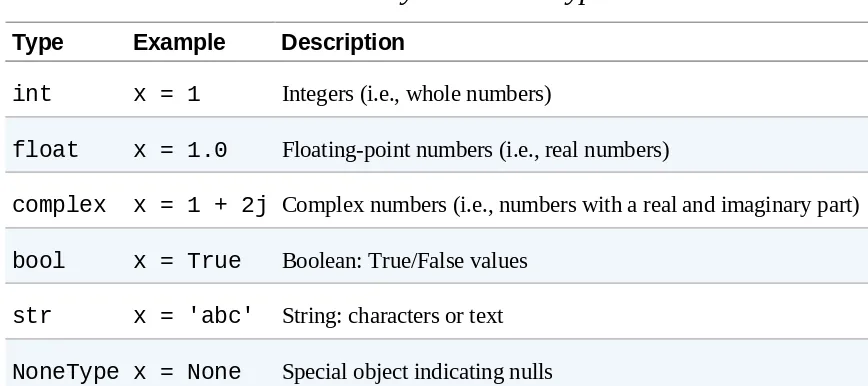
Python’s simple types are summarized in Table 1-1.
Table 1-1. Python scalar types Type Example Description
int x = 1 Integers (i.e., whole numbers)
float x = 1.0 Floating-point numbers (i.e., real numbers)
complex x = 1 + 2j Complex numbers (i.e., numbers with a real and imaginary part)
bool x = True Boolean: True/False values
str x = 'abc' String: characters or text
NoneType x = None Special object indicating nulls
Integers
The most basic numerical type is the integer. Any number without a decimal point is an integer:
In [1]: x = 1 type(x)
Out [1]: int
Python integers are actually quite a bit more sophisticated than integers in languages like C. C integers are fixed-precision, and usually overflow at some value (often near 231 or 263, depending on your system). Python integers are variable-precision, so you can do computations that would overflow in other languages:
In [2]: 2 ** 200
Out [2]:
1606938044258990275541962092341162602522202993782792835301376
Another convenient feature of Python integers is that by default, division upcasts to floating-point type:
In [3]: 5 / 2
Out [3]: 2.5
Note that this upcasting is a feature of Python 3; in Python 2, like in many statically typed languages such as C, integer division truncates any decimal and always returns an integer:
# Python 2 behavior
>>> 5 / 2 2
In [4]: 5 // 2
Out [4]: 2
Floating-Point Numbers
The floating-point type can store fractional numbers. They can be defined either in standard decimal notation, or in exponential notation:
In [5]: x = 0.000005
An integer can be explicitly converted to a float with the float constructor:
In [7]: float(1)
Out [7]: 1.0
Floating-point precision
One thing to be aware of with floating-point arithmetic is that its precision is limited, which can cause equality tests to be unstable. For example:
In [8]: 0.1 + 0.2 == 0.3
Out [8]: False
and this leads some numbers to be represented only approximately. We can see this by printing the three values to high precision:
In [9]: print("0.1 = {0:.17f}".format(0.1))
We’re accustomed to thinking of numbers in decimal (base-10) notation, so that each fraction must be expressed as a sum of powers of 10:
1/8 = 1 · 10-1 + 2 · 10-2 + 5 · 10-3
In the familiar base-10 representation, we represent this in the familiar decimal expression: 0.125.
Computers usually store values in binary notation, so that each number is expressed as a sum of powers of 2:
1/8 = 0 · 2-1 + 0 · 2-2 + 1 · 2-3
In a base-2 representation, we can write this 0.0012, where the subscript 2 indicates binary notation. The value 0.125 = 0.0012 happens to be one number which both binary and decimal notation can represent in a finite number of digits.
In the familiar base-10 representation of numbers, you are probably familiar with numbers that can’t be expressed in a finite number of digits. For
example, dividing 1 by 3 gives, in standard decimal notation: 1/3 = 0.333333333...
The 3s go on forever: that is, to truly represent this quotient, the number of required digits is infinite!
1/10 = 0.00011001100110011...2
Just as decimal notation requires an infinite number of digits to perfectly represent 1/3, binary notation requires an infinite number of digits to represent 1/10. Python internally truncates these representations at 52 bits beyond the first nonzero bit on most systems.
Complex Numbers
Complex numbers are numbers with real and imaginary (floating-point) parts. We’ve seen integers and real numbers before; we can use these to construct a complex number:
In [10]: complex(1, 2)
Out [10]: (1+2j)
Alternatively, we can use the j suffix in expressions to indicate the imaginary part:
In [11]: 1 + 2j
Out [11]: (1+2j)
Complex numbers have a variety of interesting attributes and methods, which we’ll briefly demonstrate here:
In [12]: c = 3 + 4j
In [13]: c.real # real part
Out [13]: 3.0
In [14]: c.imag # imaginary part
Out [14]: 4.0
In [15]: c.conjugate() # complex conjugate
Out [15]: (3-4j)
In [16]:
abs(c) # magnitude--that is, sqrt(c.real ** 2 + c.imag ** 2)
String Type
Strings in Python are created with single or double quotes:
In [17]: message = "what do you like?" response = 'spam'
Python has many extremely useful string functions and methods; here are a few of them:
Out [20]: 'What do you like?'
In [21]: # concatenation with +
message + response
Out [21]: 'what do you like?spam'
In [22]: # multiplication is multiple concatenation
5 * response
Out [22]: 'spamspamspamspamspam'
In [23]: # Access individual characters (zero-based indexing)
message[0]
None Type
Python includes a special type, the NoneType, which has only a single possible value: None. For example:
In [24]: type(None)
Out [24]: NoneType
You’ll see None used in many places, but perhaps most commonly it is used as the default return value of a function. For example, the print() function in Python 3 does not return anything, but we can still catch its value:
In [25]: return_value = print('abc')
abc
In [26]: print(return_value)
None
Likewise, any function in Python with no return value is, in reality, returning
Boolean Type
The Boolean type is a simple type with two possible values: True and
False, and is returned by comparison operators discussed previously:
In [27]: result = (4 < 5) result
Out [27]: True
In [28]: type(result)
Out [28]: bool
Keep in mind that the Boolean values are case-sensitive: unlike some other languages, True and False must be capitalized!
In [29]: print(True, False)
True False
Booleans can also be constructed using the bool() object constructor: values of any other type can be converted to Boolean via predictable rules. For example, any numeric type is False if equal to zero, and True otherwise:
In [30]: bool(2014)
Out [30]: True
In [31]: bool(0)
Out [31]: False
In [32]: bool(3.1415)
The Boolean conversion of None is always False:
In [33]: bool(None)
Out [33]: False
For strings, bool(s) is False for empty strings and True otherwise:
In [34]: bool("")
Out [34]: False
In [35]: bool("abc")
Out [35]: True
For sequences, which we’ll see in the next section, the Boolean representation is False for empty sequences and True for any other sequences:
In [36]: bool([1, 2, 3])
Out [36]: True
In [37]: bool([])
Built-In Data Structures
We have seen Python’s simple types: int, float, complex, bool, str, and so on. Python also has several built-in compound types, which act as containers for other types. These compound types are:
Type Name Example Description
list [1, 2, 3] Ordered collection
tuple (1, 2, 3) Immutable ordered collection
dict {'a':1, 'b':2, 'c':3} Unordered (key,value) mapping
set {1, 2, 3} Unordered collection of unique values
Lists
Lists are the basic ordered and mutable data collection type in Python. They can be defined with comma-separated values between square brackets; here is a list of the first several prime numbers:
In [1]: L = [2, 3, 5, 7]
Lists have a number of useful properties and methods available to them. Here we’ll take a quick look at some of the more common and useful ones:
In [2]: # Length of a list
In [4]: # Addition concatenates lists
L + [13, 17, 19]
In addition, there are many more built-in list methods; they are well-covered in Python’s online documentation.
contain objects of any type, or even a mix of types. For example:
In [6]: L = [1, 'two', 3.14, [0, 3, 5]]
This flexibility is a consequence of Python’s dynamic type system. Creating such a mixed sequence in a statically typed language like C can be much more of a headache! We see that lists can even contain other lists as elements. Such type flexibility is an essential piece of what makes Python code
relatively quick and easy to write.
So far we’ve been considering manipulations of lists as a whole; another essential piece is the accessing of individual elements. This is done in Python via indexing and slicing, which we’ll explore next.
List indexing and slicing
Python provides access to elements in compound types through indexing for single elements, and slicing for multiple elements. As we’ll see, both are indicated by a square-bracket syntax. Suppose we return to our list of the first several primes:
In [7]: L = [2, 3, 5, 7, 11]
Python uses zero-based indexing, so we can access the first and second element in using the following syntax:
In [8]: L[0]
Out [8]: 2
In [9]: L[1]
Out [9]: 3
Elements at the end of the list can be accessed with negative numbers, starting from -1:
Out [10]: 11
In [12]: L[-2]
Out [12]: 7
You can visualize this indexing scheme this way:
Here values in the list are represented by large numbers in the squares; list indices are represented by small numbers above and below. In this case,
L[2] returns 5, because that is the next value at index 2.
Where indexing is a means of fetching a single value from the list, slicing is a means of accessing multiple values in sublists. It uses a colon to indicate the start point (inclusive) and end point (non-inclusive) of the subarray. For example, to get the first three elements of the list, we can write it as follows:
In [12]: L[0:3]
Out [12]: [2, 3, 5]
Notice where 0 and 3 lie in the preceding diagram, and how the slice takes just the values between the indices. If we leave out the first index, 0 is assumed, so we can equivalently write the following:
In [13]: L[:3]
Out [13]: [2, 3, 5]
In [14]: L[-3:]
Out [14]: [5, 7, 11]
Finally, it is possible to specify a third integer that represents the step size; for example, to select every second element of the list, we can write:
In [15]: L[::2] # equivalent to L[0:len(L):2]
Out [15]: [2, 5, 11]
A particularly useful version of this is to specify a negative step, which will reverse the array:
In [16]: L[::-1]
Out [16]: [11, 7, 5, 3, 2]
Both indexing and slicing can be used to set elements as well as access them. The syntax is as you would expect:
In [17]: L[0] = 100
Tuples
Tuples are in many ways similar to lists, but they are defined with parentheses rather than square brackets:
In [19]: t = (1, 2, 3)
They can also be defined without any brackets at all:
In [20]: t = 1, 2, 3 print(t)
(1, 2, 3)
Like the lists discussed before, tuples have a length, and individual elements can be extracted using square-bracket indexing:
In [21]: len(t)
Out [21]: 3
In [22]: t[0]
Out [22]: 1
The main distinguishing feature of tuples is that they are immutable: this means that once they are created, their size and contents cannot be changed:
In [23]: t[1] = 4
---TypeError Traceback (most recent call last)
<ipython-input-23-141c76cb54a2> in <module>() ----> 1 t[1] = 4
In [24]: t.append(4)
---AttributeError Traceback (most recent call last)
<ipython-input-24-e8bd1632f9dd> in <module>() ----> 1 t.append(4)
AttributeError: 'tuple' object has no attribute 'append'
Tuples are often used in a Python program; a particularly common case is in functions that have multiple return values. For example, the
as_integer_ratio() method of floating-point objects returns a
numerator and a denominator; this dual return value comes in the form of a tuple:
In [25]: x = 0.125
x.as_integer_ratio()
Out [25]: (1, 8)
These multiple return values can be individually assigned as follows:
In [26]: numerator, denominator = x.as_integer_ratio() print(numerator / denominator)
0.125
Dictionaries
Dictionaries are extremely flexible mappings of keys to values, and form the basis of much of Python’s internal implementation. They can be created via a comma-separated list of key:value pairs within curly braces:
In [27]: numbers = {'one':1, 'two':2, 'three':3}
Items are accessed and set via the indexing syntax used for lists and tuples, except here the index is not a zero-based order but valid key in the dictionary:
In [28]: # Access a value via the key
numbers['two']
Out [28]: 2
New items can be added to the dictionary using indexing as well:
In [29]: # Set a new key/value pair
numbers['ninety'] = 90 print(numbers)
{'three': 3, 'ninety': 90, 'two': 2, 'one': 1}
Sets
The fourth basic collection is the set, which contains unordered collections of unique items. They are defined much like lists and tuples, except they use the curly brackets of dictionaries:
In [30]: primes = {2, 3, 5, 7} odds = {1, 3, 5, 7, 9}
If you’re familiar with the mathematics of sets, you’ll be familiar with
operations like the union, intersection, difference, symmetric difference, and others. Python’s sets have all of these operations built in via methods or operators. For each, we’ll show the two equivalent methods:
In [31]: # union: items appearing in either
primes | odds # with an operator
primes.union(odds) # equivalently with a method
Out [31]: {1, 2, 3, 5, 7, 9}
In [32]: # intersection: items appearing in both
primes & odds # with an operator
# symmetric difference: items appearing in only one set primes ^ odds # with an operator
primes.symmetric_difference(odds) # equivalently with a method
Out [34]: {1, 2, 9}
More Specialized Data Structures
Python contains several other data structures that you might find useful; these can generally be found in the built-in collections module. The
collections module is fully documented in Python’s online
documentation, and you can read more about the various objects available there.
In particular, I’ve found the following very useful on occasion:
collections.namedtuple
Like a tuple, but each value has a name
collections.defaultdict
Like a dictionary, but unspecified keys have a user-specified default value
collections.OrderedDict
Like a dictionary, but the order of keys is maintained
Control Flow
Control flow is where the rubber really meets the road in programming. Without it, a program is simply a list of statements that are sequentially executed. With control flow, you can execute certain code blocks
conditionally and/or repeatedly: these basic building blocks can be combined to create surprisingly sophisticated programs!
Here we’ll cover conditional statements (including if, elif, and else) and loop statements (including for and while, and the accompanying
Conditional Statements: if, elif, and else
Conditional statements, often referred to as if-then statements, allow the programmer to execute certain pieces of code depending on some Boolean condition. A basic example of a Python conditional statement is this:
In [1]: x = -15 if x == 0:
print(x, "is zero") elif x > 0:
print(x, "is positive") elif x < 0:
print(x, "is negative") else:
print(x, "is unlike anything I've ever seen...")
-15 is negative
Note especially the use of colons (:) and whitespace to denote separate blocks of code.
Python adopts the if and else often used in other languages; its more unique keyword is elif, a contraction of “else if”. In these conditional clauses, elif and else blocks are optional; additionally, you can
for loops
Loops in Python are a way to repeatedly execute some code statement. So, for example, if we’d like to print each of the items in a list, we can use a for
loop:
In [2]: for N in [2, 3, 5, 7]:
print(N, end=' ') # print all on same line
2 3 5 7
Notice the simplicity of the for loop: we specify the variable we want to use, the sequence we want to loop over, and use the in operator to link them together in an intuitive and readable way. More precisely, the object to the right of the in can be any Python iterator. An iterator can be thought of as a generalized sequence, and we’ll discuss them in “Iterators”.
For example, one of the most commonly used iterators in Python is the
range object, which generates a sequence of numbers:
In [3]: for i in range(10): print(i, end=' ')
0 1 2 3 4 5 6 7 8 9
You might notice that the meaning of range arguments is very similar to the slicing syntax that we covered in “Lists”.
Note that the behavior of range() is one of the differences between Python 2 and Python 3: in Python 2, range() produces a list, while in Python 3,
while loops
The other type of loop in Python is a while loop, which iterates until some condition is met:
In [6]: i = 0
while i < 10:
print(i, end=' ') i += 1
0 1 2 3 4 5 6 7 8 9
break and continue: Fine-Tuning Your Loops
There are two useful statements that can be used within loops to fine-tune how they are executed:
The break statement breaks out of the loop entirely
The continue statement skips the remainder of the current loop, and goes to the next iteration
These can be used in both for and while loops.
Here is an example of using continue to print a string of even numbers. In this case, the result could be accomplished just as well with an if-else
statement, but sometimes the continue statement can be a more convenient way to express the idea you have in mind:
In [7]: for n in range(20):
Here is an example of a break statement used for a less trivial task. This loop will fill a list with all Fibonacci numbers up to a certain value:
Loops with an else Block
One rarely used pattern available in Python is the else statement as part of a
for or while loop. We discussed the else block earlier: it executes if all the if and elif statements evaluate to False. The loop-else is perhaps one of the more confusingly named statements in Python; I prefer to think of it as a nobreak statement: that is, the else block is executed only if the loop ends naturally, without encountering a break statement.
As an example of where this might be useful, consider the following (non-optimized) implementation of the Sieve of Eratosthenes, a well-known algorithm for finding prime numbers:
In [9]: L = [] nmax = 30
for n in range(2, nmax): for factor in L:
if n % factor == 0: break
else: # no break
L.append(n) print(L)
[2, 3, 5, 7, 11, 13, 17, 19, 23, 29]
Defining and Using Functions
So far, our scripts have been simple, single-use code blocks. One way to organize our Python code and to make it more readable and reusable is to factor-out useful pieces into reusable functions. Here we’ll cover two ways of creating functions: the def statement, useful for any type of function, and the
Using Functions
Functions are groups of code that have a name and can be called using
parentheses. We’ve seen functions before. For example, print in Python 3 is a function:
In [1]: print('abc')
abc
Here print is the function name, and 'abc' is the function’s argument. In addition to arguments, there are keyword arguments that are specified by name. One available keyword argument for the print() function (in Python 3) is sep, which tells what character or characters should be used to separate multiple items:
In [2]: print(1, 2, 3)
1 2 3
In [3]: print(1, 2, 3, sep='--')
1--2--3
Defining Functions
Functions become even more useful when we begin to define our own, organizing functionality to be used in multiple places. In Python, functions are defined with the def statement. For example, we can encapsulate a
version of our Fibonacci sequence code from the previous section as follows:
In [4]: def fibonacci(N):
Now we have a function named fibonacci which takes a single argument
N, does something with this argument, and returns a value; in this case, a list of the first N Fibonacci numbers:
In [5]: fibonacci(10)
Out [5]: [1, 1, 2, 3, 5, 8, 13, 21, 34, 55]
If you’re familiar with strongly typed languages like C, you’ll immediately notice that there is no type information associated with the function inputs or outputs. Python functions can return any Python object, simple or compound, which means constructs that may be difficult in other languages are
straightforward in Python.
Default Argument Values
Often when defining a function, there are certain values that we want the function to use most of the time, but we’d also like to give the user some flexibility. In this case, we can use default values for arguments. Consider the
fibonacci function from before. What if we would like the user to be able to play with the starting values? We could do that as follows:
In [7]: def fibonacci(N, a=0, b=1):
With a single argument, the result of the function call is identical to before:
In [8]: fibonacci(10)
Out [8]: [1, 1, 2, 3, 5, 8, 13, 21, 34, 55]
But now we can use the function to explore new things, such as the effect of new starting values:
In [9]: fibonacci(10, 0, 2)
Out [9]: [2, 2, 4, 6, 10, 16, 26, 42, 68, 110]
The values can also be specified by name if desired, in which case the order of the named values does not matter:
In [10]: fibonacci(10, b=3, a=1)
*args and **kwargs: Flexible Arguments
Sometimes you might wish to write a function in which you don’t initially know how many arguments the user will pass. In this case, you can use the special form *args and **kwargs to catch all arguments that are passed. Here is an example:
characters preceding them. args and kwargs are just the variable names often used by convention, short for “arguments” and “keyword arguments”. The operative difference is the asterisk characters: a single * before a
variable means “expand this as a sequence”, while a double ** before a variable means “expand this as a dictionary”. In fact, this syntax can be used not only with the function definition, but with the function call as well!
In [14]: inputs = (1, 2, 3) keywords = {'pi': 3.14}
catch_all(*inputs, **keywords)
args = (1, 2, 3)
Anonymous (lambda) Functions
Earlier we quickly covered the most common way of defining functions, the
def statement. You’ll likely come across another way of defining short, one-off functions with the lambda statement. It looks something like this:
In [15]: add = lambda x, y: x + y
add(1, 2)
Out [15]: 3
This lambda function is roughly equivalent to
In [16]: def add(x, y): return x + y
So why would you ever want to use such a thing? Primarily, it comes down to the fact that everything is an object in Python, even functions themselves! That means that functions can be passed as arguments to functions.
As an example of this, suppose we have some data stored in a list of dictionaries:
In [17]:
data = [{'first':'Guido', 'last':'Van Rossum', 'YOB':1956}, {'first':'Grace', 'last':'Hopper', 'YOB':1906}, {'first':'Alan', 'last':'Turing', 'YOB':1912}]
Now suppose we want to sort this data. Python has a sorted function that does this:
In [18]: sorted([2,4,3,5,1,6])
Out [18]: [1, 2, 3, 4, 5, 6]
In [19]: # sort alphabetically by first name
sorted(data, key=lambda item: item['first'])
Out [19]:
[{'YOB': 1912, 'first': 'Alan', 'last': 'Turing'}, {'YOB': 1906, 'first': 'Grace', 'last': 'Hopper'}, {'YOB': 1956, 'first': 'Guido', 'last': 'Van Rossum'}]
In [20]: # sort by year of birth
sorted(data, key=lambda item: item['YOB'])
Out [20]:
[{'YOB': 1906, 'first': 'Grace', 'last': 'Hopper'}, {'YOB': 1912, 'first': 'Alan', 'last': 'Turing'},
{'YOB': 1956, 'first': 'Guido', 'last': 'Van Rossum'}]
While these key functions could certainly be created by the normal, def
Errors and Exceptions
No matter your skill as a programmer, you will eventually make a coding mistake. Such mistakes come in three basic flavors:
Syntax errors
Errors where the code is not valid Python (generally easy to fix)
Runtime errors
Errors where syntactically valid code fails to execute, perhaps due to invalid user input (sometimes easy to fix)
Semantic errors
Errors in logic: code executes without a problem, but the result is not what you expect (often very difficult to identify and fix)
Here we’re going to focus on how to deal cleanly with runtime errors. As we’ll see, Python handles runtime errors via its exception handling
Runtime Errors
If you’ve done any coding in Python, you’ve likely come across runtime errors. They can happen in a lot of ways.
For example, if you try to reference an undefined variable:
In [1]: print(Q)
---NameError Traceback (most recent call last)
<ipython-input-3-e796bdcf24ff> in <module>() ----> 1 print(Q)
NameError: name 'Q' is not defined
Or if you try an operation that’s not defined:
In [2]: 1 + 'abc'
---TypeError Traceback (most recent call last)
<ipython-input-4-aab9e8ede4f7> in <module>() ----> 1 1 + 'abc'
TypeError: unsupported operand type(s) for +: 'int' and 'str'
Or you might be trying to compute a mathematically ill-defined result:
In [3]: 2 / 0
---ZeroDivisionError Traceback (most recent call last)
ZeroDivisionError: division by zero
Or maybe you’re trying to access a sequence element that doesn’t exist:
In [4]: L = [1, 2, 3] L[1000]
---IndexError Traceback (most recent call last)
<ipython-input-6-06b6eb1b8957> in <module>() 1 L = [1, 2, 3]
----> 2 L[1000]
IndexError: list index out of range
Note that in each case, Python is kind enough to not simply indicate that an error happened, but to spit out a meaningful exception that includes
Catching Exceptions: try and except
The main tool Python gives you for handling runtime exceptions is the
try…except clause. Its basic structure is this:
In [5]:
try:
print("this gets executed first")
except:
print("this gets executed only if there is an error")
this gets executed first
Note that the second block here did not get executed: this is because the first block did not return an error. Let’s put a problematic statement in the try
block and see what happens:
Here we see that when the error was raised in the try statement (in this case, a ZeroDivisionError), the error was caught, and the except
statement was executed.
In [8]: safe_divide(1, 2)
Out [8]: 0.5
In [9]: safe_divide(2, 0)
Out [9]: 1e+100
There is a subtle problem with this code, though: what happens when another type of exception comes up? For example, this is probably not what we
intended:
In [10]: safe_divide (1, '2')
Out [10]: 1e+100
Dividing an integer and a string raises a TypeError, which our over-zealous code caught and assumed was a ZeroDivisionError! For this reason, it’s nearly always a better idea to catch exceptions explicitly:
2 try:
----> 3 return a / b
4 except ZeroDivisionError: 5 return 1E100
TypeError: unsupported operand type(s) for /: 'int' and 'str'
Raising Exceptions: raise
We’ve seen how valuable it is to have informative exceptions when using parts of the Python language. It’s equally valuable to make use of informative exceptions within the code you write, so that users of your code (foremost yourself!) can figure out what caused their errors.
The way you raise your own exceptions is with the raise statement. For example:
In [14]: raise RuntimeError("my error message")
---RuntimeError Traceback (most recent call last)
<ipython-input-16-c6a4c1ed2f34> in <module>() ----> 1 raise RuntimeError("my error message")
RuntimeError: my error message
As an example of where this might be useful, let’s return to the fibonacci
function that we defined previously:
One potential problem here is that the input value could be negative. This will not currently cause any error in our function, but we might want to let the user know that a negative N is not supported. Errors stemming from invalid parameter values, by convention, lead to a ValueError being raised:
if N < 0:
Now the user knows exactly why the input is invalid, and could even use a
try…except block to handle it!
Diving Deeper into Exceptions
Briefly, I want to mention here some other concepts you might run into. I’ll not go into detail on these concepts and how and why to use them, but instead simply show you the syntax so you can explore more on your own.
Accessing the error message
Sometimes in a try…except statement, you would like to be able to work with the error message itself. This can be done with the as keyword:
In [20]: try:
With this pattern, you can further customize the exception handling of your function.
Defining custom exceptions
In addition to built-in exceptions, it is possible to define custom exceptions through class inheritance. For instance, if you want a special kind of
ValueError, you can do this:
----> 4 raise MySpecialError("here's the message")
MySpecialError: here's the message
This would allow you to use a try…except block that only catches this type of error:
In [22]:
try:
print("do something")
raise MySpecialError("[informative error message here]")
except MySpecialError:
print("do something else")
do something do something else
try…except…else…finally
In addition to try and except, you can use the else and finally
keywords to further tune your code’s handling of exceptions. The basic structure is this:
In [23]: try:
print("try something here") except:
print("this happens only if it fails") else:
print("this happens only if it succeeds") finally:
print("this happens no matter what")
try something here
this happens only if it succeeds this happens no matter what
Iterators
Often an important piece of data analysis is repeating a similar calculation, over and over, in an automated fashion. For example, you may have a table of names that you’d like to split into first and last, or perhaps of dates that you’d like to convert to some standard format. One of Python’s answers to this is the iterator syntax. We’ve seen this already with the range iterator:
In [1]: for i in range(10): print(i, end=' ')
0 1 2 3 4 5 6 7 8 9