Practical Regression and Anova using R

(1)

Practical Regression and Anova using R

Julian J. Faraway

(2)

1

Copyright c 1999, 2000, 2002 Julian J. Faraway

(3)

Preface

There are many books on regression and analysis of variance. These books expect different levels of pre-paredness and place different emphases on the material. This book is not introductory. It presumes some knowledge of basic statistical theory and practice. Students are expected to know the essentials of statistical inference like estimation, hypothesis testing and confidence intervals. A basic knowledge of data analysis is presumed. Some linear algebra and calculus is also required.

The emphasis of this text is on the practice of regression and analysis of variance. The objective is to learn what methods are available and more importantly, when they should be applied. Many examples are presented to clarify the use of the techniques and to demonstrate what conclusions can be made. There is relatively less emphasis on mathematical theory, partly because some prior knowledge is assumed and partly because the issues are better tackled elsewhere. Theory is important because it guides the approach we take. I take a wider view of statistical theory. It is not just the formal theorems. Qualitative statistical concepts are just as important in Statistics because these enable us to actually do it rather than just talk about it. These qualitative principles are harder to learn because they are difficult to state precisely but they guide the successful experienced Statistician.

Data analysis cannot be learnt without actually doing it. This means using a statistical computing pack-age. There is a wide choice of such packages. They are designed for different audiences and have different strengths and weaknesses. I have chosen to useR(ref. Ihaka and Gentleman (1996)). Why do I useR? The are several reasons.

1. Versatility. R is a also a programming language, so I am not limited by the procedures that are preprogrammed by a package. It is relatively easy to program new methods inR.

2. Interactivity. Data analysis is inherently interactive. Some older statistical packages were designed when computing was more expensive and batch processing of computations was the norm. Despite improvements in hardware, the old batch processing paradigm lives on in their use.Rdoes one thing at a time, allowing us to make changes on the basis of what we see during the analysis.

3. R is based on S from which the commercial package S-plus is derived. R itself is open-source software and may be freely redistributed. Linux, Macintosh, Windows and other UNIX versions are maintained and can be obtained from the R-project at www.r-project.org. R is mostly compatible with S-plus meaning that S-plus could easily be used for the examples given in this book.

4. Popularity. SAS is the most common statistics package in general butR or S is most popular with researchers in Statistics. A look at common Statistical journals confirms this popularity. R is also popular for quantitative applications in Finance.

The greatest disadvantage of Ris that it is not so easy to learn. Some investment of effort is required before productivity gains will be realized. This book is not an introduction toR. There is a short introduction

(4)

3

in the Appendix but readers are referred to the R-project web site atwww.r-project.orgwhere you can find introductory documentation and information about books onR . I have intentionally included in the text all the commands used to produce the output seen in this book. This means that you can reproduce these analyses and experiment with changes and variations before fully understandingR. The reader may choose to start working through this text before learningRand pick it up as you go.

The web site for this book is at www.stat.lsa.umich.edu/˜faraway/bookwhere data de-scribed in this book appears. Updates will appear there also.

(5)

Introduction

1.1 Before you start

Statistics starts with a problem, continues with the collection of data, proceeds with the data analysis and finishes with conclusions. It is a common mistake of inexperienced Statisticians to plunge into a complex analysis without paying attention to what the objectives are or even whether the data are appropriate for the proposed analysis. Look before you leap!

1.1.1 Formulation

The formulation of a problem is often more essential than its solution which may be merely a matter of mathematical or experimental skill.Albert Einstein

To formulate the problem correctly, you must

1. Understand the physical background. Statisticians often work in collaboration with others and need to understand something about the subject area. Regard this as an opportunity to learn something new rather than a chore.

2. Understand the objective. Again, often you will be working with a collaborator who may not be clear about what the objectives are. Beware of “fishing expeditions” - if you look hard enough, you’ll almost always find something but that something may just be a coincidence.

3. Make sure you know what the client wants. Sometimes Statisticians perform an analysis far more complicated than the client really needed. You may find that simple descriptive statistics are all that are needed.

4. Put the problem into statistical terms. This is a challenging step and where irreparable errors are sometimes made. Once the problem is translated into the language of Statistics, the solution is often routine. Difficulties with this step explain why Artificial Intelligence techniques have yet to make much impact in application to Statistics. Defining the problem is hard to program.

That a statistical method can read in and process the data is not enough. The results may be totally meaningless.

(10)

1.1. BEFORE YOU START 9

1.1.2 Data Collection

It’s important to understand how the data was collected.

Are the data observational or experimental? Are the data a sample of convenience or were they obtained via a designed sample survey. How the data were collected has a crucial impact on what conclusions can be made.

Is there non-response? The data you don’t see may be just as important as the data you do see. Are there missing values? This is a common problem that is troublesome and time consuming to deal with.

How are the data coded? In particular, how are the qualitative variables represented.

What are the units of measurement? Sometimes data is collected or represented with far more digits than are necessary. Consider rounding if this will help with the interpretation or storage costs. Beware of data entry errors. This problem is all too common — almost a certainty in any real dataset of at least moderate size. Perform some data sanity checks.

1.1.3 Initial Data Analysis

This is a critical step that should always be performed. It looks simple but it is vital. Numerical summaries - means, sds, five-number summaries, correlations. Graphical summaries

– One variable - Boxplots, histograms etc. – Two variables - scatterplots.

– Many variables - interactive graphics.

Look for outliers, data-entry errors and skewed or unusual distributions. Are the data distributed as you expect?

Getting data into a form suitable for analysis by cleaning out mistakes and aberrations is often time consuming. It often takes more time than the data analysis itself. In this course, all the data will be ready to analyze but you should realize that in practice this is rarely the case.

Let’s look at an example. The National Institute of Diabetes and Digestive and Kidney Diseases conducted a study on 768 adult female Pima Indians living near Phoenix. The following variables were recorded: Number of times pregnant, Plasma glucose concentration a 2 hours in an oral glucose tolerance test, Diastolic blood pressure (mm Hg), Triceps skin fold thickness (mm), 2-Hour serum insulin (mu U/ml), Body mass index (weight in kg/(height inm2)), Diabetes pedigree function, Age (years) and a test whether the patient shows signs of diabetes (coded 0 if negative, 1 if positive). The data may be obtained from UCI

Repository of machine learning databases athttp://www.ics.uci.edu/˜mlearn/MLRepository.html. Of course, before doing anything else, one should find out what the purpose of the study was and more

(11)

> library(faraway) > data(pima)

> pima

pregnant glucose diastolic triceps insulin bmi diabetes age test

1 6 148 72 35 0 33.6 0.627 50 1

2 1 85 66 29 0 26.6 0.351 31 0

3 8 183 64 0 0 23.3 0.672 32 1

... much deleted ...

768 1 93 70 31 0 30.4 0.315 23 0

The library(faraway)makes the data used in this book available whiledata(pima)calls up this particular dataset. Simply typing the name of thedata frame,pimaprints out the data. It’s too long to show it all here. For a dataset of this size, one can just about visually skim over the data for anything out of place but it is certainly easier to use more direct methods.

We start with some numerical summaries: > summary(pima)

pregnant glucose diastolic triceps insulin

Min. : 0.00 Min. : 0 Min. : 0.0 Min. : 0.0 Min. : 0.0 1st Qu.: 1.00 1st Qu.: 99 1st Qu.: 62.0 1st Qu.: 0.0 1st Qu.: 0.0 Median : 3.00 Median :117 Median : 72.0 Median :23.0 Median : 30.5 Mean : 3.85 Mean :121 Mean : 69.1 Mean :20.5 Mean : 79.8 3rd Qu.: 6.00 3rd Qu.:140 3rd Qu.: 80.0 3rd Qu.:32.0 3rd Qu.:127.2 Max. :17.00 Max. :199 Max. :122.0 Max. :99.0 Max. :846.0

bmi diabetes age test

Min. : 0.0 Min. :0.078 Min. :21.0 Min. :0.000 1st Qu.:27.3 1st Qu.:0.244 1st Qu.:24.0 1st Qu.:0.000 Median :32.0 Median :0.372 Median :29.0 Median :0.000 Mean :32.0 Mean :0.472 Mean :33.2 Mean :0.349 3rd Qu.:36.6 3rd Qu.:0.626 3rd Qu.:41.0 3rd Qu.:1.000 Max. :67.1 Max. :2.420 Max. :81.0 Max. :1.000

Thesummary()command is a quick way to get the usual univariate summary information. At this stage, we are looking for anything unusual or unexpected perhaps indicating a data entry error. For this purpose, a close look at the minimum and maximum values of each variable is worthwhile. Starting withpregnant, we see a maximum value of 17. This is large but perhaps not impossible. However, we then see that the next 5 variables have minimum values of zero. No blood pressure is not good for the health — something must be wrong. Let’s look at the sorted values:

> sort(pima$diastolic)

[1] 0 0 0 0 0 0 0 0 0 0 0 0 0 0 0 0 0 0

[19] 0 0 0 0 0 0 0 0 0 0 0 0 0 0 0 0 0 24

[37] 30 30 38 40 44 44 44 44 46 46 48 48 48 48 48 50 50 50 ...etc...

(12)

that can easily occur. A careless statistician might overlook these presumed missing values and complete an analysis assuming that these were real observed zeroes. If the error was later discovered, they might then blame the researchers for using 0 as a missing value code (not a good choice since it is a valid value for some of the variables) and not mentioning it in their data description. Unfortunately such oversights are not uncommon particularly with datasets of any size or complexity. The statistician bears some share of responsibility for spotting these mistakes.

We set all zero values of the five variables toNAwhich is the missing value code used byR. > pima$diastolic[pima$diastolic == 0] <- NA

> pima$glucose[pima$glucose == 0] <- NA > pima$triceps[pima$triceps == 0] <- NA > pima$insulin[pima$insulin == 0] <- NA > pima$bmi[pima$bmi == 0] <- NA

The variabletestis not quantitative but categorical. Such variables are also calledfactors. However, because of the numerical coding, this variable has been treated as if it were quantitative. It’s best to designate such variables as factors so that they are treated appropriately. Sometimes people forget this and compute stupid statistics such as “average zip code”.

> pima$test <- factor(pima$test) > summary(pima$test)

0 1

500 268

We now see that 500 cases were negative and 268 positive. Even better is to use descriptive labels: > levels(pima$test) <- c("negative","positive")

> summary(pima)

pregnant glucose diastolic triceps insulin

Min. : 0.00 Min. : 44 Min. : 24.0 Min. : 7.0 Min. : 14.0 1st Qu.: 1.00 1st Qu.: 99 1st Qu.: 64.0 1st Qu.: 22.0 1st Qu.: 76.2 Median : 3.00 Median :117 Median : 72.0 Median : 29.0 Median :125.0 Mean : 3.85 Mean :122 Mean : 72.4 Mean : 29.2 Mean :155.5 3rd Qu.: 6.00 3rd Qu.:141 3rd Qu.: 80.0 3rd Qu.: 36.0 3rd Qu.:190.0 Max. :17.00 Max. :199 Max. :122.0 Max. : 99.0 Max. :846.0 NA’s : 5 NA’s : 35.0 NA’s :227.0 NA’s :374.0

bmi diabetes age test

Min. :18.2 Min. :0.078 Min. :21.0 negative:500 1st Qu.:27.5 1st Qu.:0.244 1st Qu.:24.0 positive:268 Median :32.3 Median :0.372 Median :29.0

Mean :32.5 Mean :0.472 Mean :33.2 3rd Qu.:36.6 3rd Qu.:0.626 3rd Qu.:41.0 Max. :67.1 Max. :2.420 Max. :81.0 NA’s :11.0

Now that we’ve cleared up the missing values and coded the data appropriately we are ready to do some plots. Perhaps the most well-known univariate plot is the histogram:

(13)

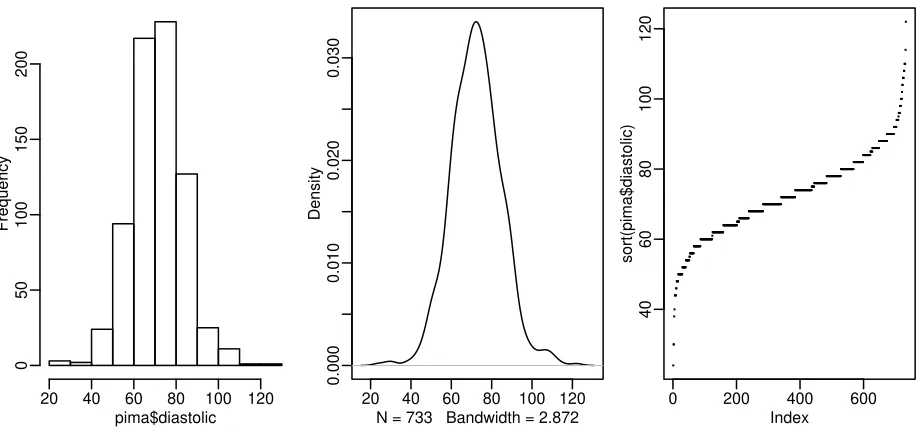
Figure 1.1: First panel shows histogram of the diastolic blood pressures, the second shows a kernel density estimate of the same while the the third shows an index plot of the sorted values

as shown in the first panel of Figure 1.1. We see a bell-shaped distribution for the diastolic blood pressures centered around 70. The construction of a histogram requires the specification of the number of bins and their spacing on the horizontal axis. Some choices can lead to histograms that obscure some features of the data. Rattempts to specify the number and spacing of bins given the size and distribution of the data but this choice is not foolproof and misleading histograms are possible. For this reason, I prefer to use Kernel Density Estimates which are essentially a smoothed version of the histogram (see Simonoff (1996) for a discussion of the relative merits of histograms and kernel estimates).

> plot(density(pima$diastolic,na.rm=TRUE))

The kernel estimate may be seen in the second panel of Figure 1.1. We see that it avoids the distracting blockiness of the histogram. An alternative is to simply plot the sorted data against its index:

plot(sort(pima$diastolic),pch=".")

The advantage of this is we can see all the data points themselves. We can see the distribution and possible outliers. We can also see the discreteness in the measurement of blood pressure - values are rounded to the nearest even number and hence we the “steps” in the plot.

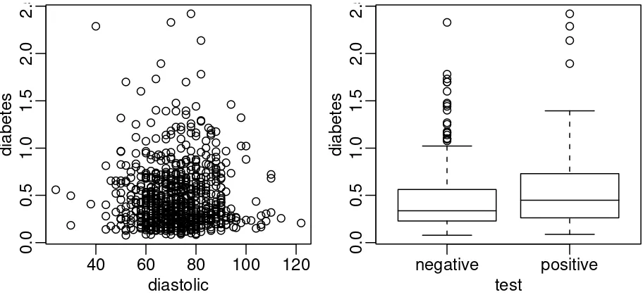
Now a couple of bivariate plots as seen in Figure 1.2: > plot(diabetes ˜ diastolic,pima) > plot(diabetes ˜ test,pima) hist(pima$diastolic)

(14)

1.2. WHEN TO USE REGRESSION ANALYSIS 13

Figure 1.2: First panel shows scatterplot of the diastolic blood pressures against diabetes function and the second shows boxplots of diastolic blood pressure broken down by test result

> pairs(pima)

We will be seeing more advanced plots later but the numerical and graphical summaries presented here are sufficient for a first look at the data.

1.2 When to use Regression Analysis

Regression analysis is used for explaining or modeling the relationship between a single variableY, called

theresponse, output ordependentvariable, and one or more predictor, input, independent orexplanatory

variables, X1✂✁✂✁✂✁✄Xp. When p

☎ 1, it is called simple regression but when p

✆

1 it is called multiple re-gression or sometimes multivariate rere-gression. When there is more than oneY, then it is called multivariate multiple regression which we won’t be covering here.

The response must be a continuous variable but the explanatory variables can be continuous, discrete or categorical although we leave the handling of categorical explanatory variables to later in the course. Taking the example presented above, a regression of diastolicand bmion diabetes would be a multiple regression involving only quantitative variables which we shall be tackling shortly. A regression of diastolicandbmiontestwould involve one predictor which is quantitative which we will consider in later in the chapter onAnalysis of Covariance. A regression ofdiastolicon justtestwould involve just qualitative predictors, a topic calledAnalysis of VarianceorANOVAalthough this would just be a simple two sample situation. A regression oftest(the response) ondiastolicandbmi(the predictors) would involve a qualitative response. Alogistic regressioncould be used but this will not be covered in this book.

Regression analyses have several possible objectives including 1. Prediction of future observations.

(15)

1.3. HISTORY 14

Extensions exist to handle multivariate responses, binary responses (logistic regression analysis) and count responses (poisson regression).

1.3 History

Regression-type problems were first considered in the 18th century concerning navigation using astronomy. Legendre developed the method of least squares in 1805. Gauss claimed to have developed the method a few years earlier and showed that the least squares was the optimal solution when the errors are normally distributed in 1809. The methodology was used almost exclusively in the physical sciences until later in the 19th century. Francis Galton coined the term regression to mediocrityin 1875 in reference to the simple regression equation in the form

y ¯y

SDy

☎ r

✁

x ¯x✂

SDx

✁

Galton used this equation to explain the phenomenon that sons of tall fathers tend to be tall but not as tall as their fathers while sons of short fathers tend to be short but not as short as their fathers. This effect is called

theregression effect.

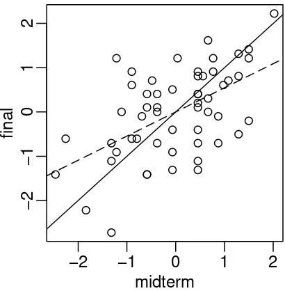
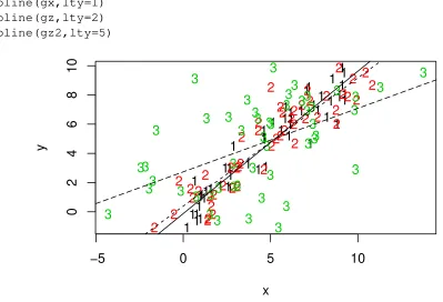
We can illustrate this effect with some data on scores from a course taught using this book. In Figure 1.3, we see a plot of midterm against final scores. We scale each variable to have mean 0 and SD 1 so that we are not distracted by the relative difficulty of each exam and the total number of points possible. Furthermore, this simplifies the regression equation to

y☎ rx

> data(stat500)

> stat500 <- data.frame(scale(stat500)) > plot(final ˜ midterm,stat500)

> abline(0,1)

−2

−1

0

1

2 −2

−1

0

1

2 midterm

final

(16)

1.3. HISTORY 15

We have added the y☎ x (solid) line to the plot. Now a student scoring, say one standard deviation

above average on the midterm might reasonably expect to do equally well on the final. We compute the least squares regression fit and plot the regression line (more on the details later). We also compute the correlations.

> g <- lm(final ˜ midterm,stat500) > abline(g$coef,lty=5)

> cor(stat500)

midterm final hw total

midterm 1.00000 0.545228 0.272058 0.84446 final 0.54523 1.000000 0.087338 0.77886 hw 0.27206 0.087338 1.000000 0.56443 total 0.84446 0.778863 0.564429 1.00000

We see that the the student scoring 1 SD above average on the midterm is predicted to score somewhat less above average on the final (see the dotted regression line) - 0.54523 SD’s above average to be exact. Correspondingly, a student scoring below average on the midterm might expect to do relatively better in the final although still below average.

If exams managed to measure the ability of students perfectly, then provided that ability remained un-changed from midterm to final, we would expect to see a perfect correlation. Of course, it’s too much to expect such a perfect exam and some variation is inevitably present. Furthermore, individual effort is not constant. Getting a high score on the midterm can partly be attributed to skill but also a certain amount of luck. One cannot rely on this luck to be maintained in the final. Hence we see the “regression to mediocrity”.

Of course this applies to any ✁

x y✂ situation like this — an example is the so-called sophomore jinx

in sports when a rookie star has a so-so second season after a great first year. Although in the father-son example, it does predict that successive descendants will come closer to the mean, it does not imply the same of the population in general since random fluctuations will maintain the variation. In many other applications of regression, the regression effect is not of interest so it is unfortunate that we are now stuck with this rather misleading name.

(17)

Chapter 2

Estimation

2.1 Example

Let’s start with an example. Suppose thatY is the fuel consumption of a particular model of car in m.p.g. Suppose that the predictors are

1. X1— the weight of the car 2. X2— the horse power 3. X3— the no. of cylinders.

X3is discrete but that’s OK. Using country of origin, say, as a predictor would not be possible within the current development (we will see how to do this later in the course). Typically the data will be available in the form of an array like this

y1 x11 x12 x13

y2 x21 x22 x23

✁✂✁✂✁ ✁✂✁✂✁

yn xn1 xn2 xn3

wherenis the number of observations orcasesin the dataset.

2.2 Linear Model

One very general form for the model would be

Y ☎ f

✁

X1 X2 X3✂✁ ε

where f is some unknown function andεis the error in this representation which is additive in this instance. Since we usually don’t have enough data to try to estimate f directly, we usually have to assume that it has some more restricted form, perhaps linear as in

Y ☎ β0 β1X1 β2X2 β3X3 ε

whereβ_i,i☎ 0 1 2 3 are unknownparameters. β0is called theinterceptterm. Thus the problem is reduced

to the estimation of four values rather than the complicated infinite dimensional f.

In a linear model theparameters enter linearly— the predictors do not have to be linear. For example

Y ☎ β0 β1X1 β2logX2 ε

(18)

2.3. MATRIX REPRESENTATION 17

is linear but

Y ☎ β0 β1X

β2

1 ε

is not. Some relationships can be transformed to linearity — for example y☎ β0x

β

1ε can be linearized by taking logs. Linear models seem rather restrictive but because the predictors can transformed and combined in any way, they are actually very flexible. Truly non-linear models are rarely absolutely necessary and most often arise from a theory about the relationships between the variables rather than an empirical investigation.

2.3 Matrix Representation

Given the actual data, we may write

yi☎ β0 β1x1i β2x2i β3x3i εi i☎ 1

✂✁✂✁✂✁✄n

but the use of subscripts becomes inconvenient and conceptually obscure. We will find it simpler both notationally and theoretically to use a matrix/vector representation. The regression equation is written as

y☎ Xβ ε

The column of ones incorporates the intercept term. A couple of examples of using this notation are the simple no predictor, mean only modely☎ µ ε

✂

We can assume thatEε☎ 0 since if this were not so, we could simply absorb the non-zero expectation for

the error into the meanµ to get a zero expectation. For the two sample problem with a treatment group having the responsey1✂✁✂✁✂✁✄ym with meanµy and control group having response z1✂✁✂✁✂✁ zn with meanµzwe

We have the regression equationy☎ Xβ ε- what estimate ofβwould best separate the systematic

com-ponentXβfrom the random componentε. Geometrically speaking,y ✡ IR

n _while_β

✡ IR

(19)

2.5. LEAST SQUARES ESTIMATION 18

Space spanned by X Fitted in p dimensions

y in n dimensions Residual in

n−p dimensions

Figure 2.1: Geometric representation of the estimationβ. The data vector Y is projected orthogonally onto the model space spanned byX. The fit is represented by projection ˆy☎ X

ˆ

βwith the difference between the fit and the data represented by the residual vector ˆε.

The problem is to findβsuch thatXβis close toY. The best choice of ˆβis apparent in the geometrical representation shown in Figure 2.4.

ˆ

βis in some sense the best estimate ofβwithin the model space. The response predicted by the model is ˆy☎ X

ˆ

βorHywhereH is an orthogonal projection matrix. The difference between the actual response and the predicted response is denoted by ˆε— the residuals.

The conceptual purpose of the model is to represent, as accurately as possible, something complex —y which isn-dimensional — in terms of something much simpler — the model which isp-dimensional. Thus if our model is successful, the structure in the data should be captured in those pdimensions, leaving just random variation in the residuals which lie in ann pdimensional space. We have

Data ☎ Systematic Structure Random Variation

ndimensions ☎ pdimensions

✁

n p✂ dimensions

2.5 Least squares estimation

The estimation ofβcan be considered from a non-geometric point of view. We might define the best estimate ofβas that which minimizes the sum of the squared errors,εTε. That is to say that the least squares estimate ofβ, called ˆβminimizes

Expanding this out, we get

yTy 2βXTy βTXTXβ

Differentiating with respect toβand setting to zero, we find that ˆβsatisfies

XTXβˆ ☎ X

T_y

These are called the normal equations. We can derive the same result using the geometric approach. Now providedXTX is invertible

(20)

2.6. EXAMPLES OF CALCULATING ˆβ 19

H☎ X

✁

XTX✂

1_XT_{is called the “hat-matrix” and is the orthogonal projection of}_y_{onto the space spanned} byX.His useful for theoretical manipulations but you usually don’t want to compute it explicitly as it is an n nmatrix.

Later we will show that the least squares estimate is the best possible estimate ofβwhen the errorsεare uncorrelated and have equal variance - i.e. varε☎ σ

2_I_.

2.6 Examples of calculating

β

ˆ

1. Wheny☎ µ ε,X ☎ 1andβ☎ µsoX

2. Simple linear regression (one predictor)

yi☎ α βxi εi

We can now apply the formula but a simpler approach is to rewrite the equation as

yi☎

Now work through the rest of the calculation to reconstruct the familiar estimates, i.e. ˆ

In higher dimensions, it is usually not possible to find such explicit formulae for the parameter estimates unlessXTXhappens to be a simple form.

2.7 Why is

β

ˆ

a good estimate?

1. It results from an orthogonal projection onto the model space. It makes sense geometrically.

2. If the errors are independent and identically normally distributed, it is the maximum likelihood esti-mator. Loosely put, the maximum likelihood estimate is the value ofβthat maximizes the probability of the data that was observed.

(21)

2.8. GAUSS-MARKOV THEOREM 20

2.8 Gauss-Markov Theorem

First we need to understand the concept of anestimable function. A linear combination of the parameters ψ☎ c

T_β_{is estimable if and only if there exists a linear combination}_aT_y_{such that}

EaTy☎ c

T_β _β

Estimable functions include predictions of future observations which explains why they are worth consid-ering. If X is of full rank (which it usually is for observational data), then all linear combinations are estimable.

Gauss-Markov theorem SupposeEε☎ 0 and varε☎ σ

2_I_{. Suppose also that the structural part of the model,}_EY

☎ Xβis correct.

Letψ☎ c

T_β_{be an estimable function, then in the class of all unbiased linear estimates of}_{ψ, ˆ}_ψ

☎ c

T_βˆ _has the minimum variance and is unique.

Proof:

We start with a preliminary calculation:

SupposeaTyis some unbiased estimate ofcTβso that

EaTy ☎ c

T_β _β

aTXβ ☎ c

T_β _β

which means thataTX ☎ c

T_{. This implies that}_c_{must be in the range space of}_XT _{which in turn implies that} cis also in the range space ofXT_X_{which means there exists a}λ_{such that}

c ☎ X

Now we can show that the least squares estimator has the minimum variance — pick an arbitrary es-timable functionaTyand compute its variance:

var

Now since variances cannot be negative, we see that var ✁

aTy✂✂✁ var

✁

cTβˆ✂

In other wordscTβˆ _{has minimum variance. It now remains to show that it is unique. There will be equality} in above relation if var ✁

aTy λTXTy✂ ☎ 0 which would require that a

T λT_XT

☎ 0 which means that

(22)

2.9. MEAN AND VARIANCE OF ˆβ 21

Implications

The Gauss-Markov theorem shows that the least squares estimate ˆβis a good choice, but if the errors are correlated or have unequal variance, there will be better estimators. Even if the errors behave but are non-normal then non-linear or biased estimates may work better in some sense. So this theorem does not tell one to use least squares all the time, it just strongly suggests it unless there is some strong reason to do otherwise.

Situations where estimators other than ordinary least squares should be considered are

1. When the errors are correlated or have unequal variance, generalized least squares should be used. 2. When the error distribution is long-tailed, then robust estimates might be used. Robust estimates are

typically not linear iny.

3. When the predictors are highly correlated (collinear), then biased estimators such as ridge regression might be preferable.

1_σ2 _{is a variance-covariance matrix. Sometimes you want the} standard error for a particular component which can be picked out as inse

✁

I H✂y. Now after some calculation, one can show

thatEεˆT_ε_ˆ

is an unbiased estimate ofσ2_. _n _p_{is the}_{degrees of freedom}_{of the model. Actually a theorem parallel to} the Gauss-Markov theorem shows that it has the minimum variance among all quadratic unbiased estimators ofσ2.

2.11 Goodness of Fit

(23)

2.11. GOODNESS OF FIT 22

0.0

0.2

0.4

0.6

0.8

1.0 −0.2

0.2

0.6

1.0 x

y

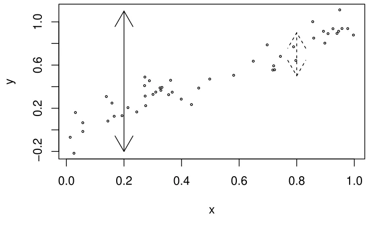
Figure 2.2: Variation in the response ywhen xis known is denoted by dotted arrows while variation iny whenxis unknown is shown with the solid arrows

The range is 0 R2 1 - values closer to 1 indicating better fits. For simple linear regressionR2☎ r

2_where ris the correlation betweenxandy. An equivalent definition is

R2☎

∑✁

ˆ

yi ¯y✂

2

∑✁

yi ¯y✂

2

The graphical intuition behindR2is shown in Figure 2.2. Suppose you want to predicty. If you don’t knowx, then your best prediction is ¯ybut the variability in this prediction is high. If you do knowx, then your prediction will be given by the regression fit. This prediction will be less variable provided there is some relationship betweenxandy.R2is one minus the ratio of the sum of squares for these two predictions. Thus for perfect predictions the ratio will be zero andR2will be one.

Warning: R2as defined here doesn’t make any sense if you do not have an intercept in your model. This

is because the denominator in the definition ofR2has a null model with an intercept in mind when the sum of squares is calculated. Alternative definitions ofR2 are possible when there is no intercept but the same graphical intuition is not available and theR2’s obtained should not be compared to those for models with an intercept. Beware of highR2’s reported from models without an intercept.

What is a good value ofR2? It depends on the area of application. In the biological and social sciences, variables tend to be more weakly correlated and there is a lot of noise. We’d expect lower values for R2 in these areas — a value of 0.6 might be considered good. In physics and engineering, where most data comes from closely controlled experiments, we expect to get much higher R2’s and a value of 0.6 would be considered low. Of course, I generalize excessively here so some experience with the particular area is necessary for you to judge yourR2’s well.

(24)

2.12. EXAMPLE 23

must understand whether the practical significance of this measure whereasR2, being unitless, is easy to understand.

2.12 Example

Now let’s look at an example concerning the number of species of tortoise on the various Galapagos Islands. There are 30 cases (Islands) and 7 variables in the dataset. We start by reading the data intoRand examining it

> data(gala) > gala

Species Endemics Area Elevation Nearest Scruz Adjacent

Baltra 58 23 25.09 346 0.6 0.6 1.84

Bartolome 31 21 1.24 109 0.6 26.3 572.33

cases deleted

---Tortuga 16 8 1.24 186 6.8 50.9 17.95

Wolf 21 12 2.85 253 34.1 254.7 2.33

The variables are

Species The number of species of tortoise found on the island

Endemics The number of endemic species

Elevation The highest elevation of the island (m)

Nearest The distance from the nearest island (km)

Scruz The distance from Santa Cruz island (km)

Adjacent The area of the adjacent island (km2)

The data were presented by Johnson and Raven (1973) and also appear in Weisberg (1985). I have filled in some missing values for simplicity (see Chapter 14 for how this can be done). Fitting a linear model inR

is done using thelm()command. Notice the syntax for specifying the predictors in the model. This is the so-calledWilkinson-Rogersnotation. In this case, since all the variables are in the gala data frame, we must use thedata=argument:

> gfit <- lm(Species ˜ Area + Elevation + Nearest + Scruz + Adjacent, data=gala)

> summary(gfit) Call:

lm(formula = Species ˜ Area + Elevation + Nearest + Scruz + Adjacent, data = gala)

Residuals:

Min 1Q Median 3Q Max

(25)

2.12. EXAMPLE 24

Coefficients:

Estimate Std. Error t value Pr(>|t|) (Intercept) 7.06822 19.15420 0.37 0.7154 Area -0.02394 0.02242 -1.07 0.2963 Elevation 0.31946 0.05366 5.95 3.8e-06 Nearest 0.00914 1.05414 0.01 0.9932 Scruz -0.24052 0.21540 -1.12 0.2752 Adjacent -0.07480 0.01770 -4.23 0.0003 Residual standard error: 61 on 24 degrees of freedom Multiple R-Squared: 0.766, Adjusted R-squared: 0.717

F-statistic: 15.7 on 5 and 24 degrees of freedom, p-value: 6.84e-07 We can identify several useful quantities in this output. Other statistical packages tend to produce output quite similar to this. One useful feature ofRis that it is possible to directly calculate quantities of interest. Of course, it is not necessary here because thelm()function does the job but it is very useful when the statistic you want is not part of the pre-packaged functions.

First we make the X-matrix

> x <- cbind(1,gala[,-c(1,2)]) and here’s the response y:

> y <- gala$Species

Now let’s constructXTX:t()does transpose and%*%does matrix multiplication: > t(x) %*% x

Error: %*% requires numeric matrix/vector arguments

Gives a somewhat cryptic error. The problem is that matrix arithmetic can only be done with numeric values butxhere derives from the data frame type. Data frames are allowed to contain character variables which would disallow matrix arithmetic. We need to force x into the matrix form:

> x <- as.matrix(x) > t(x) %*% x

Inverses can be taken using thesolve()command: > xtxi <- solve(t(x) %*% x)

> xtxi

A somewhat more direct way to get ✁

XTX✂

1_{is as follows:}

> gfit <- lm(Species ˜ Area + Elevation + Nearest + Scruz + Adjacent, data=gala)

(26)

2.12. EXAMPLE 25

The names()command is the way to see the components of an Splus object - you can see that there are other useful quantities that are directly available:

> names(gs) > names(gfit)

In particular, the fitted (or predicted) values and residuals are > gfit$fit

> gfit$res

We can get ˆβdirectly: > xtxi %*% t(x) %*% y

[,1] [1,] 7.068221 [2,] -0.023938 [3,] 0.319465 [4,] 0.009144 [5,] -0.240524 [6,] -0.074805

or in a computationally efficient and stable manner: > solve(t(x) %*% x, t(x) %*% y)

[,1] [1,] 7.068221 [2,] -0.023938 [3,] 0.319465 [4,] 0.009144 [5,] -0.240524 [6,] -0.074805

We can estimateσusing the estimator in the text: > sqrt(sum(gfit$resˆ2)/(30-6))

[1] 60.975

Compare this to the results above.

We may also obtain the standard errors for the coefficients. Also diag() returns the diagonal of a matrix):

> sqrt(diag(xtxi))*60.975

[1] 19.154139 0.022422 0.053663 1.054133 0.215402 0.017700 Finally we may compute R2:

(27)

Chapter 3

Inference

Up till now, we haven’t found it necessary to assume any distributional form for the errorsε. However, if we want to make any confidence intervals or perform any hypothesis tests, we will need to do this. The usual assumption is that the errors are normally distributed and in practice this is often, although not always, a reasonable assumption. We’ll assume that the errors are independent and identically normally distributed with mean 0 and varianceσ2, i.e.

ε N

✁

0 σ2I✂

We can handle non-identity variance matrices provided we know the form — see the section on gener-alized least squares later. Now sincey☎ Xβ ε,

y N

✁

Xβ σ2I✂

is a compact description of the regression model and from this we find that (using the fact that linear com-binations of normally distributed values are also normal)

ˆ

3.1 Hypothesis tests to compare models

Given several predictors for a response, we might wonder whether all are needed. Consider a large model, Ω, and a smaller model,ω, which consists of a subset of the predictors that are inΩ. By the principle of Occam’s Razor (also known as the law of parsimony), we’d prefer to useωif the data will support it. So we’ll take ωto represent the null hypothesis and Ωto represent the alternative. A geometric view of the problem may be seen in Figure 3.1.

If RSS_ω RSS_Ωis small, thenωis an adequate model relative toΩ. This suggests that something like RSS_ω RSS_Ω

RSS_Ω

would be a potentially good test statistic where the denominator is used for scaling purposes.

As it happens the same test statistic arises from the likelihood-ratio testing approach. We give an outline of the development: IfL

✁

β σ✁

y✂ is likelihood function, then the likelihood ratio statistic is

(28)

3.1. HYPOTHESIS TESTS TO COMPARE MODELS 27 Residual for small model

Y

Figure 3.1: Geometric view of the comparison between big model, Ω, and small model,ω. The squared length of the residual vector for the big model isRSSΩwhile that for the small model isRSSω. By Pythago-ras’ theorem, the squared length of the vector connecting the two fits isRSSω RSSΩ. A small value for this indicates that the small model fits almost as well as the large model and thus might be preferred due to its simplicity.

The test should reject if this ratio is too large. Working through the details, we find that L which gives us a test that rejects if

ˆ (constants are not the same) or

RSS_ω

which is the same statistics suggested by the geometric view. It remains for us to discover the null distribu-tion of this statistic.

Now suppose that the dimension (no. of parameters) of Ω is q and dimension of ω is p. Now by Cochran’s theorem, if the null (ω) is true then

RSS_ω RSS_Ω and these two quantities are independent. So we find that

(29)

3.2. SOME EXAMPLES 28

Thus we would reject the null hypothesis ifF ✆

F α✁

q p✂n q

The degrees of freedom of a model is (usually) the number of observations minus the number of parameters so this test statistic can be written

F ☎

also to a subspace. This test is very widely used in regression and analysis of variance. When it is applied in different situations, the form of test statistic may be re-expressed in various different ways. The beauty of this approach is you only need to know the general form. In any particular case, you just need to figure out which models represents the null and alternative hypotheses, fit them and compute the test statistic. It is very versatile.

3.2 Some Examples

3.2.1 Test of all predictors

Are any of the predictors useful in predicting the response?

Full model (Ω) :y☎ Xβ εwhereXis a full-rankn pmatrix.

Reduced model (ω) :y☎ µ ε— predictyby the mean.

We could write the null hypothesis in this case as

H0:β1☎

y ¯y✂ ☎ SYY, which is sometimes known as the sum of squares corrected for the

mean.

We’d now refer to Fp 1✂n p for a critical value or a p-value. Large values of F would indicate rejection

of the null. Traditionally, the information in the above test is presented in an analysis of variance table. Most computer packages produce a variant on this. See Table 3.1. It is not really necessary to specifically compute all the elements of the table. As the originator of the table, Fisher said in 1931, it is “nothing but a convenient way of arranging the arithmetic”. Since he had to do his calculations by hand, the table served some purpose but it is less useful now.

(30)

Source Deg. of Freedom Sum of Squares Mean Square F

Regression p 1 SSreg SSreg

✁

Table 3.1: Analysis of Variance table

When the null is rejected, this does not imply that the alternative model is the best model. We don’t know whether all the predictors are required to predict the response or just some of them. Other predictors might also be added — for example quadratic terms in the existing predictors. Either way, the overall F-test is just the beginning of an analysis and not the end.

Let’s illustrate this test and others using an old economic dataset on 50 different countries. These data are averages over 1960-1970 (to remove business cycle or other short-term fluctuations). dpiis per-capita disposable income in U.S. dollars;ddpiis the percent rate of change in per capita disposable income;sr is aggregate personal saving divided by disposable income. The percentage population under 15 (pop15) and over 75 (pop75) are also recorded. The data come from Belsley, Kuh, and Welsch (1980). Take a look at the data:

> data(savings) > savings

sr pop15 pop75 dpi ddpi Australia 11.43 29.35 2.87 2329.68 2.87 Austria 12.07 23.32 4.41 1507.99 3.93 cases deleted

---Malaysia 4.71 47.20 0.66 242.69 5.08 First consider a model with all the predictors:

> g <- lm(sr ˜ pop15 + pop75 + dpi + ddpi, data=savings) > summary(g)

Coefficients:

Estimate Std. Error t value Pr(>|t|) (Intercept) 28.566087 7.354516 3.88 0.00033 pop15 -0.461193 0.144642 -3.19 0.00260 pop75 -1.691498 1.083599 -1.56 0.12553 dpi -0.000337 0.000931 -0.36 0.71917 ddpi 0.409695 0.196197 2.09 0.04247 Residual standard error: 3.8 on 45 degrees of freedom Multiple R-Squared: 0.338, Adjusted R-squared: 0.28

F-statistic: 5.76 on 4 and 45 degrees of freedom, p-value: 0.00079 We can see directly the result of the test of whether any of the predictors have significance in the model. In other words, whetherβ1☎ β2☎ β3☎ β4☎ 0. Since the p-value is so small, this null hypothesis is rejected.

(31)

Do you know where all the numbers come from? Check that they match the regression summary above.

3.2.2 Testing just one predictor

Can one particular predictor be dropped from the model? The null hypothesis would beH0:βi ☎ 0. Set it

up like this

RSS_Ωis the RSS for the model with all the predictors of interest (pparameters). RSS_ωis the RSS for the model with all the above predictors except predictori.

The F-statistic may be computed using the formula from above. An alternative approach is to use a t-statistic for testing the hypothesis:

ti☎

and check for significance using a t distribution withn pdegrees of freedom.

However, squaring the t-statistic here, i.e.t_i2gives you the F-statistic, so the two approaches are identical. For example, to test the null hypothesis thatβ1 ☎ 0 i.e. thatp15is not significant in the full model, we

can simply observe that the p-value is 0.0026 from the table and conclude that the null should be rejected. Let’s do the same test using the general F-testing approach: We’ll need the RSS and df for the full model — these are 650.71 and 45 respectively.

and then fit the model that represents the null:

> g2 <- lm(sr ˜ pop75 + dpi + ddpi, data=savings) and compute the RSS and the F-statistic:

> sum(g2$resˆ2)

We can relate this to the t-based test and p-value by > sqrt(10.167)

[1] 3.1886

(32)

A somewhat more convenient way to compare two nested models is > anova(g2,g)

Analysis of Variance Table

Model 1: sr ˜ pop75 + dpi + ddpi

Model 2: sr ˜ pop15 + pop75 + dpi + ddpi Res.Df Res.Sum Sq Df Sum Sq F value Pr(>F)

1 46 798

2 45 651 1 147 10.2 0.0026

Understand that this test ofpop15is relative to the other predictors in the model, namelypop75, dpi andddpi. If these other predictors were changed, the result of the test may be different. This means that it is not possible to look at the effect ofpop15in isolation. Simply stating the null hypothesis asH0:β_pop15☎ 0

is insufficient — information about what other predictors are included in the null is necessary. The result of the test may be different if the predictors change.

3.2.3 Testing a pair of predictors

Suppose we wish to test the significance of variables Xj andXk. We might construct a table as shown just above and find that both variables have p-values greater than 0.05 thus indicating that individually neither is significant. Does this mean that bothXjandXkcan be eliminated from the model?Not necessarily

Except in special circumstances, dropping one variable from a regression model causes the estimates of the other parameters to change so that we might find that after droppingXj, that a test of the significance of Xkshows that it should now be included in the model.

If you really want to check the joint significance of Xj and Xk, you should fit a model with and then without them and use the general F-test discussed above. Remember that even the result of this test may depend on what other predictors are in the model.

Can you see how to test the hypothesis that bothpop75andddpimay be excluded from the model?

✁ ✂✄

Figure 3.2: Testing two predictors

(33)

3.2.4 Testing a subspace

Consider this example. Suppose thatyis the miles-per-gallon for a make of car andXj is the weight of the engine and Xk is the weight of the rest of the car. There would also be some other predictors. We might wonder whether we need two weight variables — perhaps they can be replaced by the total weight,Xj Xk. So if the original model was

y☎ β0

✁✂✁✂✁ βjXj βkXk ✁✂✁✂✁ ε

then the reduced model is

y☎ β0

✁✂✁✂✁ βl

✁

Xj Xk✂✁

✁✂✁✂✁ ε

which requires thatβj ☎ βkfor this reduction to be possible. So the null hypothesis is

H0:β_j☎ βk

This defines a linear subspace to which the general F-testing procedure applies. In our example, we might hypothesize that the effect of young and old people on the savings rate was the same or in other words that

H0:β_pop15☎ βpop75

In this case the null model would take the form

y☎ β0 βpop15

✁

pop15 pop75✂ βd pid pi βdd pidd pi ε

We can then compare this to the full model as follows: > g <- lm(sr ˜ .,savings)

> gr <- lm(sr ˜ I(pop15+pop75)+dpi+ddpi,savings) > anova(gr,g)

Model 1: sr ˜ I(pop15 + pop75) + dpi + ddpi Model 2: sr ˜ pop15 + pop75 + dpi + ddpi

Res.Df Res.Sum Sq Df Sum Sq F value Pr(>F)

1 46 674

2 45 651 1 23 1.58 0.21

The period in the first model formula is short hand for all the other variables in the data frame. The function I()ensures that the argument is evaluated rather than interpreted as part of the model formula. The p-value of 0.21 indicates that the null cannot be rejected here meaning that there is not evidence here that young and old people need to be treated separately in the context of this particular model.

Suppose we want to test whether one of the coefficients can be set to a particular value. For example, H0:β_{dd pi} ☎ 1

Here the null model would take the form:

y☎ β0 βpop15pop15 βpop75pop75 βd pid pi dd pi ε

(34)

3.3. CONCERNS ABOUT HYPOTHESIS TESTING 33

> gr <- lm(sr ˜ pop15+pop75+dpi+offset(ddpi),savings) > anova(gr,g)

Model 1: sr ˜ pop15 + pop75 + dpi + offset(ddpi) Model 2: sr ˜ pop15 + pop75 + dpi + ddpi

Res.Df Res.Sum Sq Df Sum Sq F value Pr(>F)

1 46 782

2 45 651 1 131 9.05 0.0043

We see that the p-value is small and the null hypothesis here is soundly rejected. A simpler way to test such point hypotheses is to use a t-statistic:

t☎

wherecis the point hypothesis. So in our example the statistic and corresponding p-value is > tstat <- (0.409695-1)/0.196197

> tstat [1] -3.0087 > 2*pt(tstat,45) [1] 0.0042861

We can see the p-value is the same as before and if we square the t-statistic > tstatˆ2

[1] 9.0525

we find we get the F-value. This latter approach is preferred in practice since we don’t need to fit two models but it is important to understand that it is equivalent to the result obtained using the general F-testing approach.

Can we test a hypothesis such as

H0:βjβk ☎ 1

using our general theory?

No. This hypothesis is not linear in the parameters so we can’t use our general method. We’d need to fit a non-linear model and that lies beyond the scope of this book.

3.3 Concerns about Hypothesis Testing

1. The general theory of hypothesis testing posits apopulationfrom which asampleis drawn — this is our data. We want to say something about the unknownpopulation valuesβusing estimated values

ˆ

βthat are obtained from thesampledata. Furthermore, we require that the data be generated using a

simple random sampleof the population. This sample is finite in size, while the population is infinite

in size or at least so large that the sample size is a negligible proportion of the whole. For more complex sampling designs, other procedures should be applied, but of greater concern is the case when the data is not a random sample at all. There are two cases:

(35)

names begin with the letter P. Provided there is no ethnic effect, it may be reasonable to consider this a random sample from the population defined by the entries in the phonebook. Here we are assuming the selection mechanism is effectively random with respect to the objectives of the study. An assessment of exchangeabilityis required - are the data as good as random? Other situations are less clear cut and judgment will be required. Such judgments are easy targets for criticism. Suppose you are studying the behavior of alcoholics and advertise in the media for study subjects. It seems very likely that such a sample will be biased perhaps in unpredictable ways. In cases such as this, a sample of convenience is clearly biased in which case conclusions must be limited to the sample itself. This situation reduces to the next case, where the sample is the population.

Sometimes, researchers may try to select a “representative” sample by hand. Quite apart from the obvious difficulties in doing this, the logic behind the statistical inference depends on the sample being random. This is not to say that such studies are worthless but that it would be unreasonable to apply anything more than descriptive statistical techniques. Confidence in the of conclusions from such data is necessarily suspect.

(b) The sample is the complete population in which case one might argue that inference is not required since the population and sample values are one and the same. For both regression datasets we have considered so far, the sample is effectively the population or a large and biased proportion thereof.

In these situations, we can put a different meaning to the hypothesis tests we are making. For the Galapagos dataset, we might suppose that if the number of species had no relation to the five geographic variables, then the observed response values would be randomly distributed between the islands without relation to the predictors. We might then ask what the chance would be under this assumption that an F-statistic would be observed as large or larger than one we actually observed. We could compute this exactly by computing the F-statistic for all possible (30!) permutations of the response variable and see what proportion exceed the observed F-statistic. This is a permutation test. If the observed proportion is small, then we must reject the contention that the response is unrelated to the predictors. Curiously, this proportion is estimated by the p-value calculated in the usual way based on the assumption of normal errors thus saving us from the massive task of actually computing the regression on all those computations. Let see how we can apply the permutation test to the savings data. I chose a model with just pop75anddpiso as to get a p-value for the F-statistic that is not too small.

> g <- lm(sr ˜ pop75+dpi,data=savings) > summary(g)

Coefficients:

Estimate Std. Error t value Pr(>|t|) (Intercept) 7.056619 1.290435 5.47 1.7e-06

pop75 1.304965 0.777533 1.68 0.10

dpi -0.000341 0.001013 -0.34 0.74

Residual standard error: 4.33 on 47 degrees of freedom Multiple R-Squared: 0.102, Adjusted R-squared: 0.0642

F-statistic: 2.68 on 2 and 47 degrees of freedom, p-value: 0.0791 We can extract the F-statistic as

(36)

> gs$fstat

value numdf dendf 2.6796 2.0000 47.0000

The functionsample()generates random permutations. We compute the F-statistic for 1000 randomly selected permutations and see what proportion exceed the the F-statistic for the origi-nal data:

> fstats <- numeric(1000) > for(i in 1:1000){

+ ge <- lm(sample(sr) ˜ pop75+dpi,data=savings) + fstats[i] <- summary(ge)$fstat[1]

+ }

> length(fstats[fstats > 2.6796])/1000 [1] 0.092

So our estimated p-value using the permutation test is 0.092 which is close to the normal theory based value of 0.0791. We could reduce variability in the estimation of the p-value simply by computing more random permutations. Since the permutation test does not depend on the assumption of normality, we might regard it as superior to the normal theory based value. Thus it is possible to give some meaning to the p-value when the sample is the population or for samples of convenience although one has to be clear that one’s conclusion apply only the particular sample.

Tests involving just one predictor also fall within the permutation test framework. We permute that predictor rather than the response

Another approach that gives meaning to the p-value when the sample is the population involves the imaginative concept of “alternative worlds” where the sample/population at hand is sup-posed to have been randomly selected from parallel universes. This argument is definitely more tenuous.

2. A model is usually only an approximation of underlying reality which makes the meaning of the pa-rameters debatable at the very least. We will say more on the interpretation of parameter estimates later but the precision of the statement thatβ1☎ 0 exactly is at odds with the acknowledged

approx-imate nature of the model. Furthermore, it is highly unlikely that a predictor that one has taken the trouble to measure and analyze has exactly zero effect on the response. It may be small but it won’t be zero.

This means that in many cases, we know that the point null hypothesis is false without even looking at the data. Furthermore, we know that the more data we have, the greater the power of our tests. Even small differences from zero will be detected with a large sample. Now if we fail to reject the null hypothesis, we might simply conclude that we didn’t have enough data to get a significant result. According to this view, the hypothesis test just becomes a test of sample size. For this reason, I prefer confidence intervals.

3. The inference depends on the correctness of the model we use. We can partially check the assumptions about the model but there will always be some element of doubt. Sometimes the data may suggest more than one possible model which may lead to contradictory results.

(37)

3.4. CONFIDENCE INTERVALS FORβ 36

be very easy to get statistically significant results, but the actual effects may be unimportant. Would we really care if test scores were 0.1% higher in one state than another? Or that some medication reduced pain by 2%? Confidence intervals on the parameter estimates are a better way of assessing the size of an effect. There are useful even when the null hypothesis is not rejected because they tell us how confident we are that the true effect or value is close to the null.

Even so, hypothesis tests do have some value, not least because they impose a check on unreasonable conclusions which the data simply does not support.

3.4 Confidence Intervals for

β

Confidence intervals provide an alternative way of expressing the uncertainty in our estimates. Even so, they are closely linked to the tests that we have already constructed. For the confidence intervals and regions that we will consider here, the following relationship holds. For a 100✁

1 α✂ % confidence region, any point

that lies within the region represents a null hypothesis that would not be rejected at the 100α% level while every point outside represents a null hypothesis that would be rejected. So, in a sense, the confidence region provides a lot more information than a single hypothesis test in that it tells us the outcome of a whole range of hypotheses about the parameter values. Of course, by selecting the particular level of confidence for the region, we can only make tests at that level and we cannot determine the p-value for any given test simply from the region. However, since it is dangerous to read too much into the relative size of p-values (as far as how much evidence they provide against the null), this loss is not particularly important.

The confidence region tells us about plausible values for the parameters in a way that the hypothesis test cannot. This makes it more valuable.

As with testing, we must decide whether to form confidence regions for parameters individually or simultaneously. Simultaneous regions are preferable but for more than two dimensions they are difficult to display and so there is still some value in computing the one-dimensional confidence intervals.

We start with the simultaneous regions. Some results from multivariate analysis show that

✁ and these two quantities are independent. Hence

✁

These regions are ellipsoidally shaped. Because these ellipsoids live in higher dimensions, they cannot easily be visualized.

Alternatively, one could consider each parameter individually which leads to confidence intervals which take the general form of

estimate✂

(38)

or specifically in this case:

ˆ

It’s better to consider the joint confidence intervals when possible, especially when the ˆβ are heavily correlated.

Consider the full model for the savings data. The.in the model formula stands for “every other variable in the data frame” which is a useful abbreviation.

> g <- lm(sr ˜ ., savings) > summary(g)

Coefficients:

Estimate Std. Error t value Pr(>|t|) (Intercept) 28.566087 7.354516 3.88 0.00033 pop15 -0.461193 0.144642 -3.19 0.00260 pop75 -1.691498 1.083599 -1.56 0.12553 dpi -0.000337 0.000931 -0.36 0.71917 ddpi 0.409695 0.196197 2.09 0.04247 Residual standard error: 3.8 on 45 degrees of freedom Multiple R-Squared: 0.338, Adjusted R-squared: 0.28

F-statistic: 5.76 on 4 and 45 degrees of freedom, p-value: 0.00079 We can construct individual 95% confidence intervals for the regression parameters ofpop75:

> qt(0.975,45)

Notice that this confidence interval is pretty wide in the sense that the upper limit is about 50 times larger than the lower limit. This means that we are not really that confident about what the exact effect of growth on savings really is.

Confidence intervals often have a duality with two-sided hypothesis tests. A 95% confidence interval contains all the null hypotheses that would not be rejected at the 5% level. Thus the interval for pop75 contains zero which indicates that the null hypothesisH0:β_pop75☎ 0 would not be rejected at the 5% level.

We can see from the output above that the p-value is 12.5% — greater than 5% — confirming this point. In contrast, we see that the interval forddpidoes not contain zero and so the null hypothesis is rejected for its regression parameter.

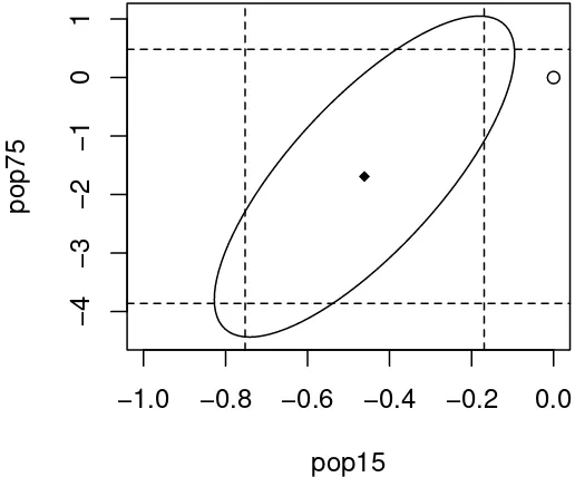
Now we construct the joint 95% confidence region for these parameters. First we load in a ”library” for drawing confidence ellipses which is not part of base R:

(39)

> plot(ellipse(g,c(2,3)),type="l",xlim=c(-1,0)) add the origin and the point of the estimates:

> points(0,0)

> points(g$coef[2],g$coef[3],pch=18)

How does the position of the origin relate to a test for removingpop75andpop15? Now we mark the one way confidence intervals on the plot for reference:

> abline(v=c(-0.461-2.01*0.145,-0.461+2.01*0.145),lty=2) > abline(h=c(-1.69-2.01*1.08,-1.69+2.01*1.08),lty=2)

See the plot in Figure 3.3.

−1.0

−0.8

−0.6

−0.4

−0.2

0.0 −4

−3

−2

−1

0

1 pop15

pop75

Figure 3.3: Confidence ellipse and regions forβ_pop75andβpop15

Why are these lines not tangential to the ellipse? The reason for this is that the confidence intervals are calculated individually. If we wanted a 95% chance that both intervals contain their true values, then the lines would be tangential.

In some circumstances, the origin could lie within both one-way confidence intervals, but lie outside the ellipse. In this case, both one-at-a-time tests would not reject the null whereas the joint test would. The latter test would be preferred. It’s also possible for the origin to lie outside the rectangle but inside the ellipse. In this case, the joint test would not reject the null whereas both one-at-a-time tests would reject. Again we prefer the joint test result.

Examine the correlation of the two predictors: > cor(savings$pop15,savings$pop75) [1] -0.90848

Practical Regression and Anova using R