Applied Statistics Using SPSS, STATISTICA, MATLAB and R

(1)

(2)

(3)

With 195 Figures and a CD

123 Joaquim P. Marques de Sá

Applied Statistics

(4)

Printed on acid-free paper SPIN: 11908944 42/ 5 4 3 2 1 0 E d itors

3100/Integra Typesettin

Production: Integra Software Services Pvt. Ltd., India Cover design: WMX design, Heidelberg

g: by the editors

Library of Congress Control Number: 2007926024

This work is subject to copyright. All rights are reserved, whether the whole or part of the material is concerned, specifically the rights of translation, reprinting, reuse of illustrations, recitation, broadcasting, reproduction on microfilm or in any other way, and storage in data banks. Duplication of this publication or parts thereof is permitted only under the provisions of the German Copyright Law of September 9, 1965, in its current version, and permission for use must always be obtained from Springer. Violations are liable for prosecution under the German Copyright Law.

Springer is a part of Springer Science+Business Media springer.com

The use of general descriptive names, registered names, trademarks, etc. in this publication does not imply, even in the absence of a specific statement, that such names are exempt from the relevant pro-tective laws and regulations and therefore free for general use.

ISBN 978-3-540-71971-7 Springer Berlin Heidelberg New York Prof. Dr. Joaquim P. Marques de Sá

Universidade do Porto Fac. Engenharia 4200-465 Porto Portugal

(5)

(6)

Preface to the Second Edition

Four years have passed since the first edition of this book. During this time I have had the opportunity to apply it in classes obtaining feedback from students and inspiration for improvements. I have also benefited from many comments by users of the book. For the present second edition large parts of the book have undergone major revision, although the basic concept – concise but sufficiently rigorous mathematical treatment with emphasis on computer applications to real datasets –, has been retained.

The second edition improvements are as follows:

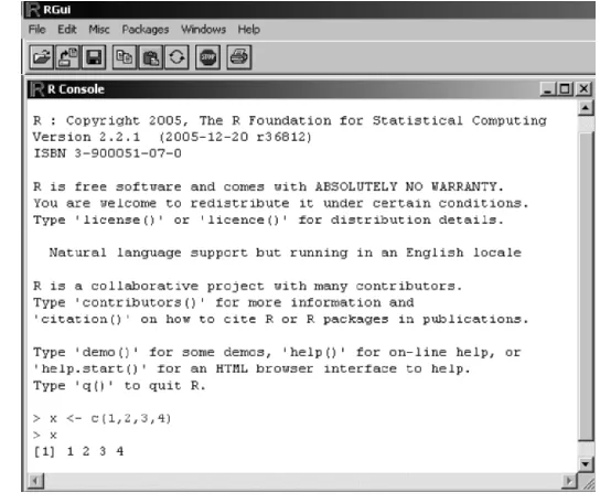
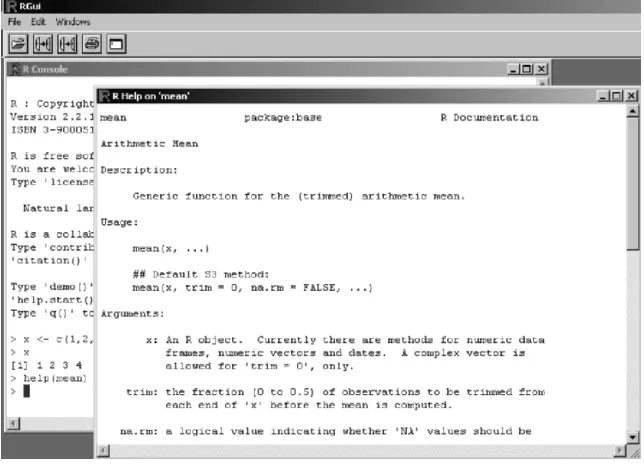
• Inclusion of R as an application tool. As a matter of fact, R is a free software product which has nowadays reached a high level of maturity and is being increasingly used by many people as a statistical analysis tool.

• Chapter 3 has an added section on bootstrap estimation methods, which have gained a large popularity in practical applications.

• A revised explanation and treatment of tree classifiers in Chapter 6 with the inclusion of the QUEST approach.

• Several improvements of Chapter 7 (regression), namely: details concerning the meaning and computation of multiple and partial correlation coefficients, with examples; a more thorough treatment and exemplification of the ridge regression topic; more attention dedicated to model evaluation.

• Inclusion in the book CD of additional MATLAB functions as well as a set of R functions.

• Extra examples and exercises have been added in several chapters. • The bibliography has been revised and new references added.

I have also tried to improve the quality and clarity of the text as well as notation. Regarding notation I follow in this second edition the more widespread use of denoting random variables with italicised capital letters, instead of using small cursive font as in the first edition. Finally, I have also paid much attention to correcting errors, misprints and obscurities of the first edition.

(14)

Preface to the First Edition

This book is intended as a reference book for students, professionals and research workers who need to apply statistical analysis to a large variety of practical problems using STATISTICA, SPSS and MATLAB. The book chapters provide a comprehensive coverage of the main statistical analysis topics (data description, statistical inference, classification and regression, factor analysis, survival data, directional statistics) that one faces in practical problems, discussing their solutions with the mentioned software packages.

The only prerequisite to use the book is an undergraduate knowledge level of mathematics. While it is expected that most readers employing the book will have already some knowledge of elementary statistics, no previous course in probability or statistics is needed in order to study and use the book. The first two chapters introduce the basic needed notions on probability and statistics. In addition, the first two Appendices provide a short survey on Probability Theory and Distributions for the reader needing further clarification on the theoretical foundations of the statistical methods described.

The book is partly based on tutorial notes and materials used in data analysis disciplines taught at the Faculty of Engineering, Porto University. One of these

management. The students in this course have a variety of educational backgrounds and professional interests, which generated and brought about datasets and analysis objectives which are quite challenging concerning the methods to be applied and the interpretation of the results. The datasets used in the book examples and exercises were collected from these courses as well as from research. They are included in the book CD and cover a broad spectrum of areas: engineering, medicine, biology, psychology, economy, geology, and astronomy.

Every chapter explains the relevant notions and methods concisely, and is illustrated with practical examples using real data, presented with the distinct intention of clarifying sensible practical issues. The solutions presented in the examples are obtained with one of the software packages STATISTICA, SPSS or MATLAB; therefore, the reader has the opportunity to closely follow what is being done. The book is not intended as a substitute for the STATISTICA, SPSS and MATLAB user manuals. It does, however, provide the necessary guidance for applying the methods taught without having to delve into the manuals. This includes, for each topic explained in the book, a clear indication of which STATISTICA, SPSS or MATLAB tools to be applied. These indications appear in

(15)

xviii Preface to the First Edition

capabilities of those software packages is also provided, which can be quite useful for practical purposes.

STATISTICA, SPSS or MATLAB do not provide specific tools for some of the statistical topics described in the book. These range from such basic issues as the choice of the optimal number of histogram bins to more advanced topics such as directional statistics. The book CD provides these tools, including a set of MATLAB functions for directional statistics.

I am grateful to many people who helped me during the preparation of the book. Professor Luís Alexandre provided help in reviewing the book contents. Professor Willem van Meurs provided constructive comments on several topics. Professor Joaquim Góis contributed with many interesting discussions and suggestions, namely on the topic of data structure analysis. Dr. Carlos Felgueiras and Paulo Sousa gave valuable assistance in several software issues and in the development of some software tools included in the book CD. My gratitude also to Professor Pimenta Monteiro for his support in elucidating some software tricks during the preparation of the text files. A lot of people contributed with datasets. Their names are mentioned in Appendix E. I express my deepest thanks to all of them. Finally, I would also like to thank Alan Weed for his thorough revision of the texts and the clarification of many editing issues.

(16)

Symbols and Abbreviations

Sample Sets A event

A set (of events)

{A1, A2,…} set constituted of events A1, A2,…

A complement of {A}

B

AU union of {A} with {B}

B

AI intersection of {A} with {B}

E set of all events (universe)

φ empty set

Functional Analysis

∃ there is

∀ for every

∈ belongs to

∉

≡ equivalent to || || Euclidian norm (vector length)

⇒

implies

→

converges to

ℜ real number set

+

ℜ [0, +∞ [

[a, b] closed interval between and including a and b

]a, b] interval between a and b, excluding a

(17)

xx Symbols and Abbreviations

]a, b[ open interval between a and b (excluding a and b)

∑

= n

i 1 sum for index i = 1,…, n

∏

= n

i 1

product for index i = 1,…, n

∫

b

a integral from a to b

k! factorial of k, k! = k(k−1)(k−2)...2.1

( )

n

k combinations of n elements taken k at a time

| x | absolute value of x

 

x largest integer smaller or equal to x gX(a) function g of variable X evaluated at a

dX dg

derivative of function g with respect to X

a n

dX g d

n derivative of order n of g evaluated at a

ln(x) natural logarithm of x

log(x) logarithm of x in base 10 sgn(x) sign of x

mod(x,y) remainder of the integer division of x by y

Vectors and Matrices

x vector (column vector), multidimensional random vector

x' transpose vector (row vector)

[x1x2…xn] row vector whose components are x1, x2,…,xn xi i-th component of vector x

xk,i i-th component of vector xk ∆x vector x increment

x'y inner (dot) product of x and y

A matrix

aij i-th row, j-th column element of matrix A A' transpose of matrix A

(18)

Symbols and Abbreviations xxi

|A| determinant of matrix A

tr(A) trace of A (sum of the diagonal elements)

I unit matrix

λi eigenvalue i

Probabilities and Distributions

X random variable (with value denoted by the same lower case letter, x)

P(A) probability of event A

P(A|B) probability of event A conditioned on B having occurred

P(x) discrete probability of random vector x P(ωi|x) discrete conditional probability of ωi given x f(x) probability density function f evaluated at x

f(x |ωi) conditional probability density function f evaluated at x given ωi

X ~ f X has probability density function f

X ~ F X has probability distribution function (is distributed as) F Pe probability of misclassification (error)

Pc probability of correct classification

df degrees of freedom

xdf,α α-percentile of X distributed with df degrees of freedom bn,p binomial probability for n trials and probability p of success Bn,p binomial distribution for n trials and probability p of success u uniform probability or density function

U uniform distribution

gp geometric probability (Bernoulli trial with probability p) Gp geometric distribution (Bernoulli trial with probability p) hN,D,n hypergeometric probability (sample of n out of N with D items) HN,D,n hypergeometric distribution (sample of n out of N with D items) pλ Poisson probability with event rate λ

Pλ Poisson distribution with event rate λ

(19)

xxii Symbols and Abbreviations

Nµ,σ normal distribution with mean µ and standard deviation σ ελ exponential density with spread factor λ

Ελ exponential distribution with spread factor λ

wα,β Weibull density with parameters α, β Wα,β Weibull distribution with parameters α, β γa,p Gamma density with parameters a, p Γa,p Gamma distribution with parameters a, p βp,q Beta density with parameters p, q Βp,q Beta distribution with parameters p, q

2 df

χ Chi-square density with df degrees of freedom

2 df

Χ Chi-square distribution with df degrees of freedom

tdf Tdf

2 1,df

df

f F density with df1, df2 degrees of freedom

2 1,df

df

F F distribution with df1, df2 degrees of freedom

Statistics

xˆ estimate of x

[ ]

X

Ε expected value (average, mean) of X

[ ]

X

V variance of X

Ε[x | y] expected value of x given y (conditional expectation)

k

m central moment of order k

µ mean value

σ standard deviation

XY

σ covariance of X and Y

ρ correlation coefficient

µ mean vector

(20)

Symbols and Abbreviations xxiii

Σ covariance matrix

x arithmetic mean

v sample variance

s sample standard deviation

xα α-quantile of X (FX(xα)=α )

med(X) median of X (same as x0.5)

S sample covariance matrix

α significance level (1−α is the confidence level)

xα α-percentile of X

ε tolerance

Abbreviations

FNR False Negative Ratio

FPR False Positive Ratio

iff if an only if

i.i.d. independent and identically distributed

IRQ inter-quartile range

pdf probability density function

LSE Least Square Error

ML Maximum Likelihood

MSE Mean Square Error

PDF probability distribution function

RMS Root Mean Square Error

r.v. Random variable

ROC Receiver Operating Characteristic

SSB Between-group Sum of Squares

SSE Error Sum of Squares

SSLF Lack of Fit Sum of Squares

SSPE Pure Error Sum of Squares

(21)

xxiv Symbols and Abbreviations

SST Total Sum of Squares

SSW Within-group Sum of Squares

TNR True Negative Ratio

TPR True Positive Ratio

VIF Variance Inflation Factor

Tradenames

EXCEL Microsoft Corporation

MATLAB The MathWorks, Inc.

SPSS SPSS, Inc.

STATISTICA Statsoft, Inc.

(22)

1 Introduction

1.1 Deterministic Data and Random Data

Our daily experience teaches us that some data are generated in accordance to known and precise laws, while other data seem to occur in a purely haphazard way.

Data generated in accordance to known and precise laws are called deterministic

gravity. When the body is released at a height h, we can calculate precisely where

the body stands at each time t. The physical law, assuming that the fall takes place

in an empty space, is expressed as:

2 0 ½gt

h

h= − ,

where h0 is the initial height and g is the Earth s gravity acceleration at the point

where the body falls.

Figure 1.1 shows the behaviour of h with t, assuming an initial height of 15

meters.

0 2 4 6 8 10 12 14 16

0 0.2 0.4 0.6 0.8 1 1.2 1.4 1.6

t

h _{t h}

0.00 15.00

0.20 14.80

0.40 14.22

0.60 13.24

0.80 11.86

1.00 10.10

1.20 7.94

1.40 5.40

1.60 2.46

Figure 1.1. Body in free-fall, with height in meters and time in seconds, assuming

g = 9.8 m/s2. The h column is an example of deterministic data.

data. An example of such type of data is the fall of a body subject to the Earth’s

(23)

2 1 Introduction

In the case of the body fall there is a law that allows the exact computation of

one of the variables h or t (for given h0 and g) as a function of the other one.

Moreover, if we repeat the body-fall experiment under identical conditions, we consistently obtain the same results, within the precision of the measurements.

These are the attributes of deterministic data: the same data will be obtained,

within the precision of the measurements, under repeated experiments in well-defined conditions.

Imagine now that we were dealing with Stock Exchange data, such as, for instance, the daily share value throughout one year of a given company. For such data there is no known law to describe how the share value evolves along the year. Furthermore, the possibility of experiment repetition with identical results does not

apply here. We are, thus, in presence of what is called random data.

Classical examples of random data are:

− Thermal noise generated in electrical resistances, antennae, etc.;

− Brownian motion of tiny particles in a fluid;

− Weather variables;

− Financial variables such as Stock Exchange share values;

− Gambling game outcomes (dice, cards, roulette, etc.);

− Conscript height at military inspection.

In none of these examples can a precise mathematical law describe the data. Also, there is no possibility of obtaining the same data in repeated experiments, performed under similar conditions. This is mainly due to the fact that several unforeseeable or immeasurable causes play a role in the generation of such data. For instance, in the case of the Brownian motion, we find that, after a certain time, the trajectories followed by several particles that have departed from exactly the same point, are completely different among them. Moreover it is found that such differences largely exceed the precision of the measurements.

When dealing with a random dataset, especially if it relates to the temporal evolution of some variable, it is often convenient to consider such dataset as one

realization (or one instance) of a set (or ensemble) consisting of a possibly infinite

number of realizations of a generating process. This is the so-called random

phenomenon composed of random parts). Thus:

− The wandering voltage signal one can measure in an open electrical

resistance is an instance of a thermal noise process (with an ensemble of infinitely many continuous signals);

− The succession of face values when tossing n times a die is an instance of a

die tossing process (with an ensemble of finitely many discrete sequences).

− The trajectory of a tiny particle in a fluid is an instance of a Brownian

process (with an ensemble of infinitely many continuous trajectories);

(24)

1.1 Deterministic Data and Random Data 3

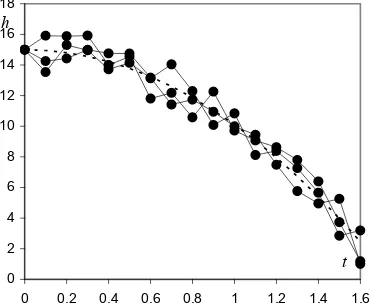
0 2 4 6 8 10 12 14 16 18

0 0.2 0.4 0.6 0.8 1 1.2 1.4 1.6

t h

1.1, with measurement errors (random data components). The dotted line

represents the theoretical curve (deterministic data component). The solid circles

correspond to the measurements made.

could probably find a deterministic description of the data. Furthermore, if we didn t know the mathematical law underlying a deterministic experiment, we might conclude that a random dataset were present. For example, imagine that we did not

experiments in the same conditions as before, performing the respective

measurement of the height h for several values of the time t, obtaining the results

shown in Figure 1.2. The measurements of each single experiment display a random variability due to measurement errors. These are always present in any dataset that we collect, and we can only hope that by averaging out such errors we

matter of fact, statistics were first used as a means of summarising data, namely

Even now the deterministic vs. random phenomenal characterization is subject to controversies and often statistical methods are applied to deterministic data. A

good example of this is the so-called chaotic phenomena, which are described by a

precise mathematical law, i.e., such phenomena are deterministic. However, the sensitivity of these phenomena on changes of causal variables is so large that the

’

Figure 1.2. Three “body fall” experiments, under identical conditions as in Figure

We might argue that if we knew all the causal variables of the “random data” we

know the “body fall” law and attempted to describe it by running several

get the “underlying law” of the data. This is a central idea in statistics: that certain quantities give the “big picture” of the data, averaging out random errors. As a social and state data (the word “statistics” coming from the “science of state”).

Scientists’ attitude towards the “deterministic vs. random” dichotomy has undergone drastic historical changes, triggered by major scientific discoveries. Paramount of these changes in recent years has been the development of the quantum description of physical phenomena, which yields a granular-all-connectedness picture of the universe. The well-known “uncertainty principle” of Heisenberg, which states a limit to our capability of ever decreasing the measurement errors of experiment related variables (e.g. position and velocity), also supports a critical attitude towards determinism.

(25)

4 1 Introduction

precision of the result cannot be properly controlled by the precision of the causes. To illustrate this, let us consider the following formula used as a model of

population growth in ecology studies, where p(n) ∈ [0, 1] is the fraction of a

limiting number of population of a species at instant n, and k is a constant that

depends on ecological conditions, such as the amount of food present:

)) 1 ( 1 (

1 n n

n p k p

p + = + − , k > 0.

Imagine we start (n = 1) with a population percentage of 50% (p1 = 0.5) and

wish to know the percentage of population at the following three time instants,

with k = 1.9:

p2 = p1(1+1.9 x (1−p1)) = 0.9750

p3 = p2(1+1.9 x (1−p2)) = 1.0213

p4 = p3(1+1.9 x (1−p3)) = 0.9800

It seems that after an initial growth the population dwindles back. As a matter of

fact, the evolution of pn shows some oscillation until stabilising at the value 1, the

limiting number of population. However, things get drastically more complicated

when k = 3, as shown in Figure 1.3. A mere deviation in the value of p1 of only

10−6 has a drastic influence on pn. For practical purposes, for k around 3 we are

unable to predict the value of the pn after some time, since it is so sensitive to very

small changes of the initial condition p1. In other words, the deterministic pn

process can be dealt with as a random process for some values of k.

a 00 10 20 30 40 50 60 70 80

0.2 0.4 0.6 0.8 1 1.2 1.4

time

p n

b 00 10 20 30 40 50 60 70 80

0.2 0.4 0.6 0.8 1 1.2 1.4

time

p _n

Figure 1.3. Two instances of the population growth process for k = 3: a) p1 = 0.1;

b) p1 = 0.100001.

The random-like behaviour exhibited by some iterative series is also present in

programs. One such routine iteratively generates xn as follows:

m x

x_n₊₁=α _nmod .

(26)

1.2 Population, Sample and Statistics 5

computing the remainder of the integer division of α times the previous number by

this purely deterministic sequence, when using numbers represented with p binary

digits, one must use m=2pand α=2p/2+3, where



p/2



is the nearest integer

smaller than p/2. The periodicity of the sequence is then 2p−2. Figure 1.4

illustrates one such sequence.

0 200 400 600 800 1000 1200

0 10 20 30 40 50 60 70 80 90 100

n xn

Figure 1.4. p =10 binary digits with m = 2p =

1024, α =35 and initial value x(0) = 2p – 3 = 1021.

1.2 Population, Sample and Statistics

When studying a collection of data as a random dataset, the basic assumption being

that no law explains any individual value of the dataset, we attempt to study the

data by means of some global measures, known as statistics, such as frequencies

(of data occurrence in specified intervals), means, standard deviations, etc.

Clearly, these same measures can be applied to a deterministic dataset, but, after all, the mean height value in a set of height measurements of a falling body, among other things, is irrelevant.

Statistics had its beginnings and key developments during the last century, especially the last seventy years. The need to compare datasets and to infer from a dataset the process that generated it, were and still are important issues addressed by statisticians, who have made a definite contribution to forwarding scientific knowledge in many disciplines (see e.g. Salsburg D, 2001). In an inferential study, from a dataset to the process that generated it, the statistician considers the dataset

as a sample from a vast, possibly infinite, collection of data called population.

Each individual item of a sample is a case (or object). The sample itself is a list of

values of one or more random variables.

The population data is usually not available for study, since most often it is either infinite or finite but very costly to collect. The data sample, obtained from

the population, should be randomly drawn, i.e., any individual in the population is

supposed to have an equal chance of being part of the sample. Only by studying

Therefore, the next number in the “random number” sequence is obtained by a suitable constant, m. In order to obtain a convenient “random-like” behaviour of

(27)

6 1 Introduction

randomly drawn samples can one expect to arrive at legitimate conclusions, about the whole population, from the data analyses.

Let us now consider the following three examples of datasets:

Example 1.1

The following Table 1.1 lists the number of firms that were established in town X during the year 2000, in each of three branches of activity.

฀

Table 1.1

Branch of Activity No. of Firms Frequencies

Commerce 56 56/109 = 51.4 %

Industry 22 22/109 = 20.2 %

Services 31 31/109 = 28.4 %

Total 109 109/109 = 100 %

Example 1.2

The following Table 1.2 lists the classifications of a random sample of 50 students in the examination of a certain course, evaluated on a scale of 1 to 5.

฀

Table 1.2

Classification No. of Occurrences Accumulated Frequencies

1 3 3/50 = 6.0%

2 10 13/50 = 26.0%

3 12 25/50 = 50.0%

4 15 40/50 = 80.0%

5 10 50/50 = 100.0%

Total 50 100.0%

Mediana = 3

a

Value below which 50% of the cases are included.

Example 1.3

The following Table 1.3 lists the measurements performed in a random sample of

10 electrical resistances, of nominal value 100 Ω (ohm), produced by a machine.

(28)

1.2 Population, Sample and Statistics 7

Table 1.3

Case # Value (in Ω)

1 101.2

2 100.3

3 99.8

4 99.8

5 99.9

6 100.1

7 99.9

8 100.3

9 99.9

10 100.1

Mean (101.2+100.3+99.8+...)/10 = 100.13

Population and sample are the same. In such a case, besides the summarization of the data by means of the frequencies of occurrence, not much more can be done. It is clearly a situation of limited interest. In the other two examples, on the other hand, we are dealing with samples of a larger population (potentially infinite in the case of Example 1.3). It s these kinds of situations that really interest the statistician – those in which the whole population is characterised based on

statistical values computed from samples, the so-called sample statistics, or just

statistics for short. For instance, how much information is obtainable about the

population mean in Example 1.3, knowing that the sample mean is 100.13 Ω?

A statistic is a function, tn, of the n sample values, xi:

) , , ,

( ₁ ₂ _n

n x x x

t K .

The sample mean computed in Table 1.3 is precisely one such function, expressed as:

∑

=

≡ n

i i

n

n x x x x n

m x

1 2

1, , , ) /

( K .

We usually intend to draw some conclusion about the population based on the statistics computed in the sample. For instance, we may want to infer about the

population mean based on the sample mean. In order to achieve this goal the xi

must be considered values of independent random variables having the same

probabilistic distribution as the population, i.e., they constitute what is called a

random sample. We sometimes encounter in the literature the expression

conveys the idea that the composition of the sample must somehow mimic the composition of the population. This is not true. What must be achieved, in order to obtain a random sample, is to simply select elements of the population at random.

’

In Example 1.1 the random variable is the “number of firms that were established in town X during the year 2000, in each of three branches of activity”.

(29)

8 1 Introduction

This can be done, for instance, with the help of a random number generator. In

statistical studies in a human population). The sampling topic is discussed in several books, e.g. (Blom G, 1989) and (Anderson TW, Finn JD, 1996). Examples of statistical malpractice, namely by poor sampling, can be found in (Jaffe AJ, Spirer HF, 1987). The sampling issue is part of the planning phase of the statistical investigation. The reader can find a good explanation of this topic in (Montgomery DC, 1984) and (Blom G, 1989).

In the case of temporal data a subtler point has to be addressed. Imagine that we are presented with a list (sequence) of voltage values originated by thermal noise in an electrical resistance. This sequence should be considered as an instance of a random process capable of producing an infinite number of such sequences. Statistics can then be computed either for the ensemble of instances or for the time sequence of the voltage values. For instance, one could compute a mean voltage value in two different ways: first, assuming one has available a sample of voltage sequences randomly drawn from the ensemble, one could compute the mean

voltage value at, say, t = 3 seconds, for all sequences; and, secondly, assuming one

such sequence lasting 10 seconds is available, one could compute the mean voltage value for the duration of the sequence. In the first case, the sample mean is an

estimate of an ensemble mean (at t = 3 s); in the second case, the sample mean is

an estimate of a temporal mean. Fortunately, in a vast number of situations,

corresponding to what are called ergodic random processes, one can derive

ensemble statistics from temporal statistics, i.e., one can limit the statistical study to the study of only one time sequence. This applies to the first two examples of random processes previously mentioned (as a matter of fact, thermal noise and dice tossing are ergodic processes; Brownian motion is not).

1.3 Random Variables

A random dataset presents the values of random variables. These establish a

mapping between an event domain and some conveniently chosen value domain

(often a subset of ℜ). A good understanding of what the random variables are and

which mappings they represent is a preliminary essential condition in any statistical analysis. A rigorous definition of a random variable (sometimes abbreviated to r.v.) can be found in Appendix A.

Usually the value domain of a random variable has a direct correspondence to the outcomes of a random experiment, but this is not compulsory. Table 1.4 lists random variables corresponding to the examples of the previous section. Italicised capital letters are used to represent random variables, sometimes with an identifying subscript. The Table 1.4 mappings between the event and the value domain are:

XF: {commerce, industry, services} → {1, 2, 3}.

XE: {bad, mediocre, fair, good, excellent} → {1, 2, 3, 4, 5}.

XR: [90 Ω, 110 Ω] → [90, 110].

(30)

1.3 Random Variables 9

Table 1.4

Dataset Variable Value Domain Type

Firms in town X, year 2000 XF {1, 2, 3} a

Discrete, Nominal

Classification of exams XE {1, 2, 3, 4, 5} Discrete, Ordinal

Electrical resistances (100 Ω) XR [90, 110] Continuous a

1 ≡ Commerce, 2 ≡ Industry, 3 ≡ Services.

One could also have, for instance:

XF: {commerce, industry, services} → {−1, 0, 1}.

XE: {bad, mediocre, fair, good, excellent} → {0, 1, 2, 3, 4}.

XR: [90 Ω, 110 Ω] → [−10, 10].

The value domains (or domains for short) of the variables XF and XE are

discrete. These variables are discrete random variables. On the other hand,

variable XR is a continuous random variable.

The values of a nominal (or categorial) discrete variable are mere symbols (even

if we use numbers) whose only purpose is to distinguish different categories (or classes). Their value domain is unique up to a biunivocal (one-to-one)

transformation. For instance, the domain of XF could also be codified as {A, B, C}

or {I, II, III}.

Examples of nominal data are:

– Class of animal: bird, mammal, reptile, etc.;

– Automobile registration plates;

– Taxpayer registration numbers.

The only statistics that make sense to compute for nominal data are the ones that are invariable under a biunivocal transformation, namely: category counts; frequencies (of occurrence); mode (of the frequencies).

The domain of ordinal discrete variables, as suggested by the name, supports a

monotonic transformation (i.e., preserving the total order relation). That is why the

domain of XE could be {0, 1, 2, 3, 4} or {0, 25, 50, 75, 100} as well.

Examples of ordinal data are abundant, since the assignment of ranking scores to items is such a widespread practice. A few examples are:

total order relation (“larger than” or “smaller than”). It is unique up to a strict

(31)

10 1 Introduction

Several statistics, whose only assumption is the existence of a total order relation, can be applied to ordinal data. One such statistic is the median, as shown in Example 1.2.

Continuous variables have a real number interval (or a reunion of intervals) as domain, which is unique up to a linear transformation. One can further distinguish

between ratio type variables, supporting linear transformations of the y = ax type,

and interval type variables supporting linear transformations of the y = ax + b type. The domain of ratio type variables has a fixed zero. This is the most frequent type of continuous variables encountered, as in Example 1.3 (a zero ohm resistance is a zero resistance in whatever measurement scale we choose to elect). The whole panoply of statistics is supported by continuous ratio type variables. The less common interval type variables do not have a fixed zero. An example of interval

type data is temperature data, which can either be measured in degrees Celsius (XC)

or in degrees Fahrenheit (XF), satisfying the relation XF = 1.8XC + 32. There are

only a few, less frequent statistics, requiring a fixed zero, not supported by this type of variables.

Notice that, strictly speaking, there is no such thing as continuous data, since all data can only be measured with finite precision. If, for example, one is dealing

1.82 m may be used. Of course, if the highest measurement precision is the millimetre, one is in fact dealing with integer numbers such as 182 mm, i.e., the height data is, in fact, ordinal data. In practice, however, one often assumes that there is a continuous domain underlying the ordinal data. For instance, one often assumes that the height data can be measured with arbitrarily high precision. Even for rank data such as the examination scores of Example 1.2, one often computes an average score, obtaining a value in the continuous interval [0, 5], i.e., one is implicitly assuming that the examination scores can be measured with a higher precision.

1.4 Probabilities and Distributions

The process of statistically analysing a dataset involves operating with an appropriate measure expressing the randomness exhibited by the dataset. This

measure is the probability measure. In this section, we will introduce a few topics

of Probability Theory that are needed for the understanding of the following material. The reader familiar with Probability Theory can skip this section. A more detailed survey (but still a brief one) on Probability Theory can be found in Appendix A.

1.4.1 Discrete Variables

The beginnings of Probability Theory can be traced far back in time to studies on chance games. The work of the Swiss mathematician Jacob Bernoulli (1654-1705),

Ars Conjectandi, represented a keystone in the development of a Theory of

(32)

1.4 Probabilities and Distributions 11

Probability, since for the first time, mathematical grounds were established and the application of probability to statistics was presented. The notion of probability is

originally associated with the notion of frequency of occurrence of one out of k

events in a sequence of trials, in which each of the events can occur by pure chance.

Let us assume a sample dataset, of size n, described by a discrete variable, X.

Assume further that there are k distinct values xi of X each one occurring ni times.

We define:

– Absolute frequency of xi: ni ;

– Relative frequency (or simply frequency of xi):

∑

= =

= k

i i i

i n n

n n f

1

with .

In the classic frequency interpretation, probability is considered a limit, for large

n, of the relative frequency of an event: P_i≡P(X =x_i)=lim_n_→_∞ f_i∈

[ ]

0,1. In

Appendix A, a more rigorous definition of probability is presented, as well as properties of the convergence of such a limit to the probability of the event (Law of

Large Numbers), and the justification for computing P(X =x_i) as the ratio of the

number of favourable events over the number of possible events when the event composition of the random experiment is known beforehand. For instance, the probability of obtaining two heads when tossing two coins is ¼ since only one out of the four possible events (head-head, head-tail, tail-head, tail-tail) is favourable. As exemplified in Appendix A, one often computes probabilities of events in this way, using enumerative and combinatorial techniques.

The values of Pi constitute the probability function values of the random

variable X, denoted P(X). In the case the discrete random variable is an ordinal

variable the accumulated sum of Pi is called the distribution function, denoted

F(X). Bar graphs are often used to display the values of probability and distribution

functions of discrete variables.

Let us again consider the classification data of Example 1.2, and assume that the frequencies of the classifications are correct estimates of the respective probabilities. We will then have the probability and distribution functions represented in Table 1.5 and Figure 1.5. Note that the probabilities add up to 1 (total certainty) which is the largest value of the monotonic increasing function

F(X).

Table 1.5. Probability and distribution functions for Example 1.2, assuming that the frequencies are correct estimates of the probabilities.

xi Probability Function P(X) Distribution Function F(X)

1 0.06 0.06

2 0.20 0.26

3 0.24 0.50

4 0.30 0.80

5 0.20 1.00

(33)

12 1 Introduction

Figure 1.5. Probability and distribution functions for Example 1.2, assuming that the frequencies are correct estimates of the probabilities.

Several discrete distributions are described in Appendix B. An important one,

since it occurs frequently in statistical studies, is the binomial distribution. It

trial is denoted p. The complementary probability of the failure is 1 – p, also

denoted q. Details on this distribution can be found in Appendix B. The respective

probability function is:

k

1.4.2 Continuous Variables

We now consider a dataset involving a continuous random variable. Since the variable can assume an infinite number of possible values, the probability associated to each particular value is zero. Only probabilities associated to intervals of the variable domain can be non-zero. For instance, the probability that a gunshot hits a particular point in a target is zero (the variable domain is here

.

For a continuous variable, X (with value denoted by the same lower case letter,

x), one can assign infinitesimal probabilities ∆p(x) to infinitesimal intervals ∆x:

x

For a finite interval [a, b] we determine the corresponding probability by adding

up the infinitesimal contributions, i.e., using:

∫

describes the probability of occurrence of a “success” event k times, in n

independent trials, performed in the same conditions. The complementary “failure” event occurs, therefore, n – k times. The probability of the “success” in a single

(34)

1.5 Beyond a Reasonable Doubt... 13

Therefore, the probability density function, f(x), must be such that:

∫

=

D f(x)dx 1, where D is the domain of the random variable.

Similarly to the discrete case, the distribution function, F(x), is now defined as:

∫

−∞

random variable to which respect the density and distribution functions.

The reader may wish to consult Appendix A in order to learn more about continuous density and distribution functions. Appendix B presents several

important continuous distributions, including the most popular, the Gauss (or

normal) distribution, with density function defined as:

2

This function uses two parameters, µ and σ, corresponding to the mean and

standard deviation, respectively. In Appendices A and B the reader finds a description of the most important aspects of the normal distribution, including the reason of its broad applicability.

1.5 Beyond a Reasonable Doubt...

Consider, for instance, the dataset of Example 1.3 and the statement the 100 Ω

electrical resistances, manufactured by the machine, have a (true) mean value in the interval [95, 105] . If one could measure all the resistances manufactured by

the machine during its whole lifetime, one could compute the population mean

(true mean) and assign a True or False value to that statement, i.e., a conclusion with entire certainty would then be established. However, one usually has only

available a sample of the population; therefore, the best one can produce is a

conclusion of the type … have a mean value in the interval [95, 105] with

probability δ ; i.e., one has to deal not with total certainty but with a degree of

certainty:

P(mean ∈[95, 105]) = δ = 1 – α .

We call δ (or1–α ) the confidence level (α is the error or significance level)

and will often present it in percentage (e.g. δ = 95%). We will learn how to

establish confidence intervals based on sample statistics (sample mean in the above

We often see movies where the jury of a Court has to reach a verdict as to whether the accused is found “guilty” or “not guilty”. The verdict must be consensual and established beyond any reasonable doubt. And like the trial jury, the statistician has also to reach objectively based conclusions, “beyond any reasonable doubt”…

“ ”

”

(35)

14 1 Introduction

example) and on appropriate models and/or conditions that the datasets must

satisfy.

Let us now look in more detail what a confidence level really means. Imagine that in Example 1.2 we were dealing with a random sample extracted from a population of a very large number of students, attending the course and subject to an examination under the same conditions. Thus, only one random variable plays a role here: the student variability in the apprehension of knowledge. Consider,

= + + =

50 10 15 12 ˆ

p 0.74.

The question is how reliable this estimate is. Since the random variable representing such an estimate (with random samples of 50 students) takes value in a continuum of values, we know that the probability that the true mean is exactly that particular value (0.74) is zero. We then loose a bit of our innate and candid faith in exact numbers, relax our exigency, and move forward to thinking in terms

of intervals around pˆ (interval estimate). We now ask with which degree of

certainty (confidence level) we can say that the true proportion p of students with

deviation – or tolerance – of ε = ±0.02 from that estimated proportion?

In order to answer this question one needs to know the so-called sampling

distribution of the following random variable:

n X P_n =(

∑

n_i₌₁ _i)/ ,

well approximated by the normal distribution with mean equal to p and standard

deviation equal to p(1−p)/n. This topic is discussed in detail in Appendices A

moment, it will suffice to say that using the normal distribution approximation (model), one is able to compute confidence levels for several values of the

tolerance, ε, and sample size, n, as shown in Table 1.6 and displayed in Figure 1.6.

Two important aspects are illustrated in Table 1.6 and Figure 1.6: first, the

confidence level always converges to 1 (absolute certainty) with increasing n;

second, when we want to be more precise in our interval estimates by decreasing

the tolerance, then, for fixed n, we have to lower the confidence levels, i.e.,

simultaneous and arbitrarily good precision and certainty are impossible (some

said the degree of certainty increases with the number of evidential facts (tending

further, that we wanted to statistically assess the statement “the student performance is 3 or above”. Denoting by p the probability of the event “the student performance is 3 or above” we derive from the dataset an estimate of p, known as

point estimate and denotedpˆ, as follows:

“performance 3 or above” is, for instance, between 0.72 and 0.76, i.e., with a

where the Xi are n independent random variables whose values are 1 in case of “success” (student performance ≥ 3 in this example) and 0 in case of “failure”.

When the np and n(1–p) quantities are “reasonably large” Pn has a distribution

and B, where what is meant by “reasonably large” is also presented. For the

(36)

1.5 Beyond a Reasonable Doubt... 15

to absolute certainty if this number tends to infinite), and that if the jury wanted to increase the precision (details) of the verdict, it would then lose in degree of certainty.

Table 1.6. Confidence levels (δ) for the interval estimation of a proportion, when

pˆ = 0.74, for two different values of the tolerance (ε).

n δ for ε = 0.02 δ for ε = 0.01

50 0.25 0.13

100 0.35 0.18

1000 0.85 0.53

10000 ≈ 1.00 0.98

0.0 0.2 0.4 0.6 0.8 1.0 1.2

0 500 1000 1500 2000 2500 3000 3500 4000

n

δ

ε=0.04

ε=0.02

ε=0.01

Figure 1.6. Confidence levels for the interval estimation of a proportion, when

pˆ = 0.74, for three different values of the tolerance.

There is also another important and subtler point concerning confidence levels.

Consider the value of δ = 0.25 for a ε = ±0.02 tolerance in the n = 50 sample size

situation (Table 1.6). When we say that the proportion of students with

performance ≥ 3 lies somewhere in the interval pˆ ± 0.02, with the confidence

level 0.25, it really means that if we were able to infinitely repeat the experiment of

randomly drawing n = 50 sized samples from the population, we would then find

that 25% of the times (in 25% of the samples) the true proportion p lies in the

interval pˆ_k± 0.02, where the pˆ (_k k = 1, 2,…) are the several sample estimates

(37)

16 1 Introduction

to obtain the 95% confidence level, for an ε = ±0.02 tolerance. It turns out to be

n≈ 1800. We now have a sample of 1800 drawings of a ball from the urn, with an

estimated proportion, saypˆ₀, of the success event. Does this mean that when

dealing with a large number of samples of size n = 1800 with estimates pˆ (_k k = 1,

2,…),95% of the pˆ will lie somewhere in the interval _k pˆ₀± 0.02? No. It means,

as previously stated and illustrated in Figure 1.7, that 95% of the intervals pˆ_k±

0.02 will contain p. As we are (usually) dealing with a single sample, we could be

1.7. Now, it is clear that 95% of the time p does not fall in thepˆ₃± 0.02 interval.

lower the risk we run in basing our conclusions on atypical samples. Assuming we increased the confidence level to 0.99, while maintaining the sample size, we

would then pay the price of a larger tolerance, ε = 0.025. We can figure this out by

imagining in Figure 1.7 that the intervals would grow wider so that now only 1 out

of 100 intervals does not contain p.

The main ideas of this discussion around the interval estimation of a proportion can be carried over to other statistical analysis situations as well. As a rule, one has to fix a confidence level for the conclusions of the study. This confidence level is intimately related to the sample size and precision (tolerance) one wishes in the conclusions, and has the meaning of a risk incurred by dealing with a sampling process that can always yield some atypical dataset, not warranting the conclusions. After losing our innate and candid faith in exact numbers we now lose a bit of our certainty about intervals…

p

#1 #2

#3

#4

#5 #6

#100 #99

...

p1 ^

− ε p1 ^

+ ε p^1

Figure 1.7. Interval estimation of a proportion. For a 95% confidence level only roughly 5 out of 100 samples, such as sample #3, are atypical, in the sense that the

respective pˆ±ε interval does not contain p.

The choice of an appropriate confidence level depends on the problem. The 95% value became a popular figure, and will be largely used throughout the book,

Imagine then that we were dealing with random samples from a random experiment in which we knew beforehand that a “success” event had a p = 0.75 probability of occurring. It could be, for instance, randomly drawing balls with replacement from an urn containing 3 black balls and 1 white “failure” ball. Using the normal approximation of Pn, one can compute the needed sample size in order

(38)

1.6 Statistical Significance and Other Significances 17

ε < 0.05) for a not too large sample size (say, n > 200), and it works well in many

applications. For some problem types, where a high risk can have serious consequences, one would then choose a higher confidence level, 99% for example.

either an infinitely large, useless, tolerance, or an infinitely large, prohibitive, sample. A compromise value achieving a useful tolerance with an affordable sample size has to be found.

1.6 Statistical Significance and Other Significances

Statistics is surely a recognised and powerful data analysis tool. Because of its recognised power and its pervasive influence in science and human affairs people tend to look to statistics as some sort of recipe book, from where one can pick up a recipe for the problem at hand. Things get worse when using statistical software and particularly in inferential data analysis. A lot of papers and publications are

People tend to lose any critical sense even in such a risky endeavour as trying to reach a general conclusion (law) based on a data sample: the inferential or inductive reasoning.

In the book of A. J. Jaffe and Herbert F. Spirer (Jaffe AJ, Spirer HF 1987) many misuses of statistics are presented and discussed in detail. These authors identify four common sources of misuse: incorrect or flawed data; lack of knowledge of the subject matter; faulty, misleading, or imprecise interpretation of the data and results; incorrect or inadequate analytical methodology. In the present book we concentrate on how to choose adequate analytical methodologies and give precise interpretation of the results. Besides theoretical explanations and words of caution the book includes a large number of examples that in our opinion help to solidify the notions of adequacy and of precise interpretation of the data and the results.

The other two sources of misuse − flawed data and lack of knowledge of the

subject matter – are the responsibility of the practitioner.

In what concerns statistical inference the reader must exert extra care of not applying statistical methods in a mechanical and mindless way, taking or using the software results uncritically. Let us consider as an example the comparison of foetal heart rate baseline measurements proposed in Exercise 4.11. The heart rate

minute, bpm), after discarding rhythm acceleration or deceleration episodes. The comparison proposed in Exercise 4.11 respects to measurements obtained in 1996 against those obtained in other years (CTG dataset samples). Now, the popular

two-sample t-test presented in chapter 4 does not detect a statiscally significant

diference between the means of the measurements performed in 1996 and those performed in other years. If a statistically significant diference was detected did it mean that the 1996 foetal population was different, in that respect, from the

because it usually achieves a “reasonable” tolerance in our conclusions (say,

Notice that arbitrarily small risks (arbitrarily small “reasonable doubt”) are often impractical. As a matter of fact, a zero risk − no “doubt” at all − means, usually,

plagued with the “computer dixit” syndrome when reporting statistical results.

(39)

18 1 Introduction

population of other years? Common sense (and other senses as well) rejects such a claim. If a statistically significant difference was detected one should look carefully to the conditions presiding the data collection: can the samples be considered as being random?; maybe the 1996 sample was collected in at-risk foetuses with lower baseline measurements; and so on. As a matter of fact, when dealing with large samples even a small compositional difference may sometimes produce statistically significant results. For instance, for the sample sizes of the CTG dataset even a difference as small as 1 bpm produces a result usually

considered as statistically significant (p = 0.02). However, obstetricians only attach

practical meaning to rhythm differences above 5 bpm; i.e., the statistically significant difference of 1 bpm has no practical significance.

Inferring causality from data is even a riskier endeavour than simple comparisons. An often encountered example is the inference of causality from a statistically significant but spurious correlation. We give more details on this issue in section 4.4.1.

One must also be very careful when performing goodness of fit tests. A common example of this is the normality assessment of a data distribution. A vast quantity of papers can be found where the authors conclude the normality of data distributions based on very small samples. (We have found a paper presented in a congress where the authors claimed the normality of a data distribution based on a sample of four cases!) As explained in detail in section 5.1.6, even with 25-sized samples one would often be wrong when admitting that a data distribution is normal because a statistical test didn t reject that possibility at a 95% confidence level. More: one would often be accepting the normality of data generated with asymmetrical and even bimodal distributions! Data distribution modelling is a difficult problem that usually requires large samples and even so one must bear in mind that most of the times and beyond a reasonable doubt one only has evidence

of a model; the true distribution remains unknown.

Another misuse of inferential statistics arrives in the assessment of classification or regression models. Many people when designing a classification or regression model that performs very well in a training set (the set used in the design) suffer from a kind of love-at-first-sight syndrome that leads to neglecting or relaxing the evaluation of their models in test sets (independent of the training sets). Research literature is full with examples of improperly validated models that are later on dropped out when more data becomes available and the initial optimism plunges down. The love-at-first-sight is even stronger when using computer software that automatically searches for the best set of variables describing the model. The book of Chamont Wang (Wang C, 1993), where many illustrations and words of caution on the topic of inferential statistics can be found, mentions an experiment where 51 data samples were generated with 100 random numbers each and a regression

dependent variable) as a function of the other ones (playing the role of independent variables). The search finished by finding a regression model with a significant

R-square and six significant coefficients at 95% confidence level. In other words, a

functional model was found explaining a relationship between noise and noise! Such a model would collapse had proper validation been applied. In the present

’