an introduction to combinatorial families–with Maple programming
Herbert S. Wilf
University of Pennsylvania Philadelphia, PA, USA
May 28, 2002
Contents
1 Introduction 4
1.1 What this is about . . . 4
2 About programming in Maple 5 2.1 Exercises . . . 8
3 Sets and subsets 9 3.1 What they are . . . 9
3.2 How many there are . . . 9
3.3 Probabilities and averages . . . 10
3.4 k-subsets . . . 12
3.5 East side, west side,. . . (I) . . . 13
3.6 Making lists and random choices of sets and subsets . . . 14
3.7 Ranking sets and subsets . . . 17
3.8 Unranking sets and subsets . . . 19
3.9 Exercises . . . 20
4 Permutations and their cycles 23 4.1 What permutations are . . . 23
4.2 What cycles are . . . 23
4.3 Counting permutations by cycles . . . 24
4.4 East side, west side ... (II) . . . 25
4.5 The generating function . . . 26
4.6 The average number of cycles . . . 27
4.7 An application . . . 28
4.8 Making lists and random choices of permutations and their cycles . . 31
4.9 Ranking permutations by cycles . . . 33
4.10 Exercises . . . 34
4.11 Maple Programming Exercises . . . 34
5 Set partitions 36 5.1 What set partitions are . . . 36
5.2 Counting set partitions by classes . . . 36
5.3 East side, west side ... (III) . . . 37
5.5 An application . . . 39
5.6 Making lists and random choices of set partitions . . . 41
5.7 Ranking set partitions . . . 43
5.8 Exercises . . . 43
6 Integer partitions 44 6.1 What they are . . . 44
6.2 East side, west side ... (IV) . . . 44
6.3 Exercises . . . 46
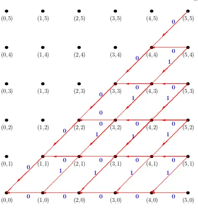
7 . . . and all around the town 47 7.1 k-subsets and codewords . . . 50
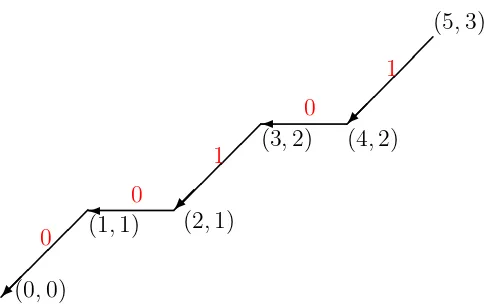
7.2 Toll charges on the roads . . . 52
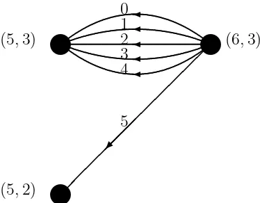
7.3 A look at one more family . . . 53
8 Some review problems 57
9 The EastWest Maple package 58
1
Introduction
1.1
What this is about
This material is intended for a course that will combine a study of combinatorial structures with introductory recursive programming in Maple.
Maple is a system for doing mathematics on a computer. It is widely available in colleges and universities. Most often Maple is used interactively. That is, you ask it a question, like
> 2+2;
and it immediately gives you the answer, in this case 4
But programming is a different kettle of fish altogether. In programming you ask the computer to carry out a sequence of instructions (program) that you have written, and the computer then retires to its cave and does so. It will report back to you when it has finished, but in the meantime it might be doing millions of things that you asked it to do, while you will have been eating chocolates and reading a novel.
So programming is a very nontrivial way to relate to a computer. But recursive
programming raises the stakes once again. A recursive program is one that calls itself in order to get the job done. Something like looking up the word horse in a dictionary, and finding that it means horse, and actually learning something from that exchange. Many high level computer languages are not capable of dealing with recursive programs, and none of them would be suitable for use in a course such as this one. Among languages that do permit recursive programming, one might ask, “Why choose Maple? Why not C++
?”
Indeed, Maple is not nearly as elegant a programming language as C++
, and a bunch of others that we might mention. In fact Maple is fairly creaky in a number of respects. But there one thing you’ll have to admit: Maple is a brilliant mathe-matician. It not only knows how to answer your questions interactively, and it not only provides a fully equipped, if cranky, computer programming language; it also knows an absolutely startling quantity of higher mathematics. C++
doesn’t know any of that. For instance, some of the tasks for which we’ll write programs below are already built-in to the Maple language.
That’s why Maple.
But why recursive? Anything that can be programmed recursively can also be pro-grammed nonrecursively. In fact, nonrecursive programs often run much faster, and are often more efficient, than recursive programs. But this is not primarily a course about writing fast and efficient programs. It is about concepts. If a mathematical object has an intrinsically recursive structure, then we will respect that structure by writing a recursive program to build it. In such cases, the recursive programs will often have great elegance and will faithfully mirror the evolution of the structures, without letting it get hidden in a sea of bookkeeping and accounting.
Recursion is very much underrepresented in mathematics curricula these days. One good way to get the subject out of hiding is by coupling it with a mathematical discussion of some structures that are inherently recursive, as are the combinatorial families in this work.
Finally, an excellent book on the nuts and bolts of Maple programming [PG] is now available. We recommend the use of that work in conjunction with this course.
These notes express a point of view that emerged while Albert Nijenhuis and I were writing Combinatorial Algorithms [NW], and specifically while we were writing the second edition of same. Indeed, if you are familiar with that volume then you will recognize that these notes cover much of the same ground as that work, adjusted for changes in programming languages and fashions, and reflecting my current predilec-tion for using recursion whenever it is natural to do so. To that collaborapredilec-tion with Albert Nijenhuis I owe most of what I know about this subject. Jim Propp made a number of comments that have improved the exposition.
2
About programming in Maple
These lecture notes are not primarily about Maple programming. They are intended to be used together with a good exposition of the Maple programming language. Since there aren’t many good books about that subject (one is [PG]), we will say a few words here about Maple, and the programs will say a few more words.
The heart of writing a Maple program is in writing a Maple procedure. A proce-dure is like a little box with a certain number of input quantities and some output quantities. It is intended to be entirely self-contained so that other programs can freely use it. A Maple procedure begins with lines like
Here findit is the name of the procedure. The input and output quantities are x,y,z,.... The variables var1, var2, ... are declared to be local variables. Local variables are variables that are used inside your procedure findit, and by declaring them to be local you are assuring that their names will not conflict with other names that are used in the programs that use your procedure findit. For instance, lots of programs use a variable named i as a summation variable. If you declare i to be local to your procedure then even though a variable named i might also appear in the main program that is using your procedure, their will be no conflict between their names. Any change that is made to the external variableiwill not affect the one that is internal to procedurefinditand conversely. Generally speaking, it is good programming practice to declare every variable that occurs inside your procedure to be local, except for the input and output variables x,y,z,..., so they will not affect other parts of the program.
Here is a Maple procedure addthemwhose mission in life is to add up the members of a given list and return the sum.
addthem:=proc(x) local i;
RETURN(add(x[i],i=1..nops(x))); end:
In this procedure, x is the input list, and the variable i is declared to be local. In that way, the external program that uses this procedure can also name variables asi, if it wishes to, and they will not conflict with the ones that are local to this procedure findit. To use this routine to add up the numbers in the list [3,1,8,19], just type > addthem([3,1,8,19]);
in a Maple worksheet, for instance, and Maple will reply 31
The next one is a recursive Maple procedure that will calculate n!. fact:=proc(n):
# Computes n factorial
Recursive programs have a certain spare beauty. Notice that this one gets its answer by calling itself with a lower value ofn, and then multiplying by n.
Here is a recursive program that will calculate the gcd of two given positive integers m and n. It expresses the mathematical fact that the gcd of m and n is the same as the gcd ofnand mmodn. Thusgcd(18,14) =gcd(14,4) =gcd(4,2) =gcd(2,0) = 2. The Maple program is the following.
gcdiv:=proc(m,n):
# Finds the gcd of two given integers
if n=0 then RETURN(m) else RETURN(gcdiv(n,m mod n)) fi: end:
A list, in Maple, consists of a left bracket, a number of items separated by commas, and a right bracket. Thus, yy:=[a,g,379,ww,sam,94] is a Maple list. If tt is a list, then its successive entries arett[1], tt[2], ..., so thatyy[3]is 379, for instance. The number of items in a list tt isnops(tt). For example, nops(yy) is 6.
A few more rarefied Maple instructions that will be of much use to us here are the following.
1. The op command. If you give to the op command a bracketed list, such as [2,1,5], it will strip off the outermost brackets, leaving the bare sequence. Thus op([9,3,17]) gives 9,3,17.
2. We can augment a list by using the op command. Suppose we have the list xx:=[1,2,3,4]; and we want to make it into the list [1,2,3,4,8]. This can be done by executing the commandy:=[op(xx),8], in which the inneropstrips off the brackets, then we adjoin the 8, and then we enclose the result in a new pair of brackets to achieve the desired effect.
3. The map command is a powerful way to distribute the effect of a function throughout a list. If we have a function, say the function
> f:=x->x^2;
and we give the command
> map(f,[1,2,3,4]); then the result will be the list [1,4,9,16]
4. Another command of this kind is applyop. This is similar to map, except that it applies the mapping only to one chosen part of the object list instead of to all. More precisely, the instruction applyop(f,j,zz); will apply the mapping f only to the jth element of zz. For example,
> applyop(x->x^2,2,[1,2,3,4]);
[1,4,3,4]
and since applyop(u->u^2,2,t)will square the 2nd entry of a given list t, we can map it too, with results like this:
> map(t->applyop(u->u^2,2,t),[[1,2,3],[1,4,5],[4,4,6]]);
[[1,4,3],[1,16,5],[4,16,6]]
2.1
Exercises
Write the following programs as self contained Maple procedures. In each case debug the program, run it on the sample problem, and hand in the program itself and the printed output.
1. Write procedure sumcoeff whose input is a polynomial in x, as an expression, and whose output is the sum of the absolute values of the coefficients of all of the powers of x in that polynomial. Run sumcoeff(3*x^2+5*x-7), for which your program should return the value 15.
2. Write a procedure sumsqdiv whose input is a positive integer n and whose output is the sum of the squares of the divisors of n including 1 and n itself. Test your program by running sumsqdiv(12) and checking the answer.
3. Write revlist, a Maple procedure whose input is a list and whose output is the same list in reverse order. Try your program by calling for
revlist([[a,b],[3,q],[1,h]]);.
5. Explain the error message that you will get if you run try(3); where the procedure try is the following:
try:=proc(x) local zz; x:=x^2+1; zz:=3; RETURN(zz); end:
3
Sets and subsets
3.1
What they are
We discuss only finite sets. A set is a collection of objects. The setS ={1,2,3,4}is the collection of those four objects. No significance is attached to the order in which the elements of a set are listed. Thus S = {1,2,3}= {1,3,2}= {3,1,2} are all the same set. A set is like a club: all that matters is whether you are a member or not.
The set of no objects at all is the empty set, written ∅. A subset T of a set S, written T ⊆ S, is a set all of whose elements are also members of S, e.g., {1,3} ⊆ {1,2,3,4}, and∅ ⊆S is true whatever the set S might be.
3.2
How many there are
The empty set has exactly one subset: itself. The setS ={1}of 1 object has exactly two subsets, namely ∅and {1}. In general, how many subsets does a set of n objects have?
Let’s gather a little more data first. If f(n) is the answer then we have already noted that f(0) = 1 and f(1) = 2. The reader will quickly check that f(2) = 4 and f(3) = 8, so our sequence of values of f(n) begins as 1,2,4,8, . . .. Well, the next valuemight be 611, but we would bet on 16. In fact, it is starting to look suspiciously as if a set S of n objects has exactly f(n) = 2n subsets, for each n= 0,1,2, . . ..
But why?
fate of 1, we move on to 2. Shall we put 2 into the subset that we are building, or not? That decision also can be made in two ways. So both of these decisions, the one that affects 1 and the one that affects 2, can be made in four ways. Similarly, we can decide whether 3 shall or shall not be in the subset that we’re making in two ways, and two ways for 4, likewise. So this set S of four elements has 16 subsets, one corresponding to each way that we make all four of the decisions that affect the memberships of 1,2,3 and 4.
Theorem 3.1 For each n = 0,1,2, . . ., the set Sn = {1,2, . . . , n} has exactly 2n
subsets.
Proof. Clearly true for n = 0. Ifn >0 then Sn has two kinds of subsets, those that
do contain n (east-side sets) and those that don’t (west-side sets). Evidently there are equal numbers of these two kinds of sets since if we delete n from an east-side set we get a west-side set, and this mapping is 1-1. But by induction, there are 2n−1
east-side sets. Thus there are 2·2n−1
= 2n subsets altogether.
✷
Example 3.1. Suppose T ⊆ {1,2, . . . , n}. We’ll define the spread s(T) of T to be the largest element ofT minus its smallest element. So s({3,4,7}) = 4, for instance. OK, for a fixed integers n > 1 and 1≤s ≤n−1, how many subsets of {1,2, . . . , n}
have spread s?
If the smallest element of such a subset is m, then the largest is m +s, for 1≤ m ≤n−s. What about the other elements of such a subset? They can be any subset at all of the set {m+ 1, m+ 2, . . . , m+s−1}, so there are 2s−1
such subsets for every m, 1 ≤ m ≤ n−s, making a total of (n−s)2s−1
subsets of {1,2, . . . , n}
that have spread s. ✷
3.3
Probabilities and averages
Continuing the example above, what is theprobability that a randomly chosen subset T ⊆ {1,2, . . . , n} will have spread s? It is the number of subsets of spread s divided by the number of subsets, i.e., (n−s)2s−1
/2n= (n−s)2s−1−n. Thus, for each n >1
and 1≤s≤n−1, the probability ps that a subset has spread s is
ps= (n−s)2s−
1−n. (n >1; 1 ≤s≤n−1) (3.1)
Suppose that students’ scores, on a scale of 1-10, from a certain exam are 7,4,5,5,8,9,6,8,5,4,1,6,4,7,6,9,9,7,10,3,5.
How might we calculate the class average? The straightforward way would be to add up all of the scores and divide by the number of scores, to get
7 + 4 + 5 + 5 + 8 + 6 + 8 + 5 + 4 + 1 + 6 + 4 + 7 + 6 + 9 + 9 + 7 + 10 + 3 + 5 20
= 119
20 = 5.95.
After doing this for a few times you would quickly learn to group the data before calculating. You would say that one student got a 1, none got a 2, one score was 3, there were three 4’s, four 5’s, three 6’s, three 7’s, two 8’s, two 9’s and one 10. Therefore the average is
1·1 + 0·2 + 1·3 + 3·4 + 4·5 + 3·6 + 3·7 + 2·8 + 2·9 + 1·10
20 = 5.95,
as before.
In the numerator of the grouped method of finding the average, we see the sum of each integer times the frequency with which it occurred, and in the denominator is the total number of students. So if for eachj = 0,1,2, . . . ,10, the number of students who got grade j was nj, then this formula says that the average is
P10
j=0jnj
N =
10
X
j=0
j n
j
N
where N =P
jnj is the total number of students. But in this formula we recognize
the quantity in parentheses, nj/N, as the probability that a student will get a score
of j. So the grouped formula for finding the average score is average =X
j
jpj. (3.2)
So what is the average spread of a subset of{1,2, ..., n}? The probability of spread s is given by (3.1), so by (3.2) the average spread is
¯ s(n) =
n−1
X
s=1
This sum can actually be expressed in a simple, closed form. To do this without1
having to think about it, you can open a Maple worksheet and type simplify(sum(s∗(n−s)∗2ˆ(s−1−n),s=1..n−1));
Maple will respond with n−3 + (n+ 3)2−n as the value of the sum. The average
spread of a subset of {1,2, . . . , n} is therefore very close ton−3.
3.4
k
-subsets
A k-subset of a set S is a subset whose cardinality is k. The 2-subsets of {1,2,3,4}
are {1,2},{1,3},{1,4},{2,3},{2,4},{3,4}. There are six of them. In general, the number is given by the following theorem.
Theorem 3.2 A set of n objects has exactly nk=n!/(k!(n−k)!) k-subsets.
To see why this is so, ask first in how many ways we can make anordered selection of k elements from a set of n elements. The first element can be chosen in n ways, the second inn−1 ways, . . ., thekth inn−k+ 1 ways, so thek-tuple can be chosen in
n(n−1)(n−2). . .(n−k+ 1) = n! (n−k)!
different ways. Now every k-subset gives rise to k! different ordered selections, one for each way of arranging its members. Hence the number of k-subsets is equal to the number of ordered selections divided by k!, which is n!/(k!(n−k)!), or nk, as claimed.
The numbers nk (“n choose k”) are the famous binomial coefficients. If n is a nonnegative integer, then the binomial coefficient nk vanishes if k < 0 or k > n.
Ifn is any real number then the binomial coefficient is well-defined as long as k is a nonnegative integer. Indeed
n k !
= n!
k!(n−k)! =
n(n−1)(n−2). . .(n−k+ 1)
k! ,
1
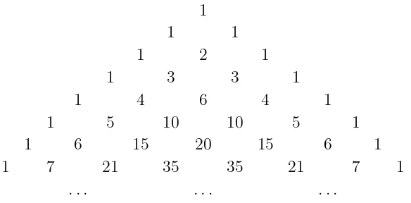
1
Figure 3.1: The Pascal triangle of binomial coefficients
and that makes perfect sense even if, say, n =−3/4. For example,
−3
The binomial coefficients can be nicely displayed in a triangular array called Pas-cal’s triangle. The rows are indexed by n = 0,1,2,3, . . ., and in the nth row of Pascal’s triangle there are the numbers n0
A quick glance at Pascal’s triangle suggests that each entry in it is the sum of the two entries that are northeast and northwest of it. In symbols, what we see is that
n
There are many ways to prove this, but the one that we will use is the east-side-west-side paradigm, because the same method will work on a variety of problems that we will encounter later.
ground. If a certain subset does not contain the letter n, then move it to the east side of town, and if it does contain n then move it to the west side.
Now instead of one large collection of subsets all over the place, we have two nice neat piles, one on the east side, and the other on the west side of town.
How many subsets are on the east side? These are the ones that don’t have n in them. Since they don’t have n then they must all be subsets of {1,2,3. . . , n−1}.
How many subsets are on the west side? These are the ones that do have n in them. If such a k-subset does contain n, what must the rest of the elements of the subset be? Evidently they must be some (k−1)-subset of{1,2, . . . , n−1}, and there since every k-subset landed on one side of town or the other. ✷
That proof was perhaps a bit more complicated than this particular situation requires, but it has the advantage that it will apply in numerous similar situations.
3.6
Making lists and random choices of sets and subsets
The counting arguments are directly wired to algorithms for making lists and for choosing objects at random.
Consider the question of making a list of all subsets of{1,2, . . . , n}. We discovered that there are 2n of these by observing that a subset can be described by giving the
status of each possible element {1,2, . . . , n} as “in” or “out”. This can conveniently be done with a vector of 0’s and 1’s, where a 1 means that the element is in, and a 0 means it is out, of the subset under consideration. Thus 0001 is the subset {4} of
{1,2,3,4}, while 1010 is the subset {1,3} and 0000 is the empty subset.
For instance, the list L(1) is [[0],[1]]. So, for n = 2, we first glue a 0 onto the beginning of each member ofL(1), getting[[0,0],[0,1]], and next we glue a 1 onto the beginning of each member ofL(1), which gives[[1,0],[1,1]]. NowL(2) is the union of these two lists, namely L(2) =[[0,0],[0,1],[1,0],[1,1]]. A Maple program2
that performs this task is as follows.
GlueIt:=(z,d)->[d,op(z)]: Subsets:=proc(n)
local east, west ; options remember; if n=0 then RETURN([[]])
else
east:=map(GlueIt,Subsets(n-1),0); west:=map(GlueIt,Subsets(n-1),1); RETURN([op(east),op(west)])
fi; end:
If we call this program with > Subsets(3)
for instance, then Maple will reply with
[[0,0,0],[0,0,1],[0,1,0],[0,1,1],[1,0,0],[1,0,1],[1,1,0],[1,1,1]] (3.5) Next suppose we want to choose a subset of {1,2, . . . , n} uniformly at random (uar), i.e., in such a way that each of the 2n possible subsets will have an equal
chance of being selected. That’s easy too. Just choose a random integer, using your random number generator, in the range 0,1, . . . ,2n−1, and express it as a binary
string of 0’s and 1’s, and you’re all done. Equivalently, toss a fair coinn times. After the ith toss, put the letter i into the random subset that is under construction if the coin came up as Heads, and leaveiout of the subset if it landed as Tails. Note that in Maple, a call torandreturns a function for generating random numbers, rather than the random numbers themselves. A Maple program3
for choosing a random subset of
{1,2, . . . , n} is shown below. 2
See the program notes on page 62.
3
RandSub:=proc(n) local rn, set, i; rn:=rand(0..1): set:=[]:
for i from 1 to n do set:=[op(set),rn()] od: RETURN(set):
end:
So much for all subsets of n things. Let’s turn now to subsets of given cardinality k (“k-subsets”). With k-subsets we can also use the east side-west side method. To make a list L(n, k) of all k-subsets of an n-set we recursively make the lists L(n−
1, k−1) and L(n−1, k). The desired list L(n, k) is obtained by beginning with the listL(n−1, k) and following that by the list that is obtained by adjoining the element n to each member of L(n−1, k−1). Let’s write that symbolically as
L(n, k) =L(n−1, k), L(n−1, k−1)⊗n. (3.6) To implement that in Maple, we will represent each subset by a list of its members. Here is a procedure4
that will list all of the k-subsets of {1,2, . . . , n}.
westop:=(y,m)->[op(y),m]: ListKSubsets:=proc(n,k)
local east,west ; options remember;
#Returns a list of the k-subsets of {1,2,...,n} if n<0 or k<0 or k>n then RETURN([])
elif n=0 or k=0 then RETURN([[]]) else
east:=ListKSubsets(n-1,k);west:=ListKSubsets(n-1,k-1); west:=map(westop,west,n);
RETURN([op(east),op(west)]); fi;
end:
For example, a call toListKSubsets(5,3) produces the response
[[1,2,3],[1,2,4],[1,3,4],[2,3,4],[1,2,5],[1,3,5],[2,3,5],[1,4,5],[2,4,5],[3,4,5]]. (3.7) 4
To choose, uniformly at random, ak-subset of{1, . . . , n}, here’s what to do: With probabilityn−1
k−1
/nk=k/nchoose uar a (k−1)-subset of {1, . . . , n−1} and adjoin n to it, or with probability 1−k/n, simply output a randomly chosen k-subset of
{1, . . . , n−1}. The Maple program5
follows.
RandomKSubsets:=proc(n,k) local rno,east,west ;
if n<0 or k<0 or k>n then RETURN()
elif n=0 and k=0 then RETURN([]) else
rno:=10^(-12)*rand(); if rno<k/n then
east:=RandomKSubsets(n-1,k-1); RETURN([op(east),n])
else
west:=RandomKSubsets(n-1,k); RETURN(west)
fi;fi; end:
3.7
Ranking sets and subsets
Suppose we have a list: {horse, turtle, cow, pig}. The rank of an element of the list is simply its position in the list, with however one technical ingredient added: the ranks start at 0. Thus, in the list above, the rank of “horse” is 0, the rank of “turtle” is 1, the rank of cow is 2 and the rank of “pig” is 3.
For a somewhat more realistic example, in the list (3.7), the rank of [1,2,3] is 0, and the rank of [2,3,4] is 3.
The ranking problem is this: given an element of a list, find its rank in that list. Of course if the list itself has actually been computed already then we can find the rank of an element just by searching for it in the list. In the ranking problems that we consider here, one should think of the lists as not having been already computed, and we are being asked to find the rank of a given element in a list even though the list is not available.
Example: What’s the rank of the subset [3,4,7,9] in the list of all of the 210
subsets of {1,2,3, . . . ,10}?
To answer this, first observe that we are representing (“encoding”) subsets by strings of 0’s and 1’s. This particular subset is therefore the string {0011001010}.
5
Next, the way we listed the subsets was that we first listed all of the strings that begin with a 0 and then we listed all that begin with a 1. Now here’s the key point: this string ss begins with a 0. Therefore it occurs in the first half of the list, and its position in that first half is the same as the rank of the truncated string ss’:={011001010} in the shorter list of all subsets of{2,3, . . . ,10}.
But now suppose that the given string ss begins with a 1, say ss:={1011001010}.
Then it lies in the second half of the full list L(10), and what is its rank in that full list? Well, all of the 29
strings that begin with a 0 precede it in the full list. So its rank is 29
plus the rank of the truncated string ss′ :={011001010}.
The beauty of the recursive view of the world is that we don’t have to say “con-tiuing in this way,” or “and so on,” at this point. Instead we can just leave it at that and write out a formal scheme for ranking a given string of n 0’s and 1’s in the list L(n).
Letss be the given string, let ss′ denote the truncation of ss that is obtained by
deleting its leading 0 or 1, and let rank(ss, L(n)) denote the rank of ss in the list L(n). If the first bit of ss is a 0, then
rank(ss, L(n)) = rank(ss′
, L(n−1)), while if the first bit is a 1 then
rank(ss, L(n)) = 2n−1
+ rank(ss′
, L(n−1)).
Thus we have the following Maple program for computing the rank of a subset. The subset is input as an array of 0’s and 1’s.
truncate:=ss->[op(2..nops(ss),ss)]: RankSubset:=proc(ss)
#Finds the rank of subset ss in the list L(nn), where #nn is the length of the array ss.
local nn; nn:=nops(ss);
if nn=0 then RETURN(0)
elif ss[1]=0 then RETURN(RankSubset(truncate(ss))) else RETURN(RankSubset(truncate(ss))+2^(nn-1)) fi;
Now we can answer the question that was posed in the example above. To find the rank of the subset [3,4,7,9] in the list of all of the 210
subsets of {1,2,3, . . . ,10}, we call
RankSubset([0,0,1,1,0,0,1,0,1,0]).
Maple returns 202, so this is the subset of rank 202 in the list, which is to say that [3,4,7,9] is the 203rdsubset in the list of all 1024 subsets of {1,2,3, . . . ,10}.
Now we turn to ranking k-subsets. Given some k-subsetS, what is the rank of S in the list of all nk k-subsets of {1,2,3, . . . , n}? But, in exactly which list of those k-subsets? The list that we’ll have in mind is the list L(n, k) that is produced by ListKSubsets above.
In that listL(n, k), all of thek-subsets that do not contain the lettern precede all of the subsets that do contain n. But that says it all. So to find the rank of a given k-subsetS inL(n, k),we ask if n ∈S or not. If n /∈S, then the rank of our set is the same as its rank in the smaller listL(n−1, k) of all k-subsets of {1,2, . . . , n−1}. If, on the other hand, n ∈ S, then let S′ = S\{n}. The rank of S in L(n, k) is n−1
k
plus the rank of S′ inL(n−1, k−1). The Maple program is as follows.
cutn:=w->[op(1..nops(w)-1,w)]; RankKSubset:=proc(ss,n,k);
#Finds the rank of the k-subset ss in the list of all #k-subsets of 1,...,n. ss is given as a list of members.
if k=0 then RETURN(0) elif ss[k]=n
then RETURN(RankKSubset(cutn(ss),n-1,k-1)+binomial(n-1,k)) else RETURN(RankKSubset(ss,n-1,k))
fi: end:
Now if we call
> RankKSubset([1,2,5],5,3);
Maple responds with 4, in agreement with eq. (3.7).
3.8
Unranking sets and subsets
certain list. In unranking we are given an integer r and a list, and we are asked to find the object whose rank is r on that list.
For instance, which is the subset of rank 784 in the list of all subsets of 13 objects? To answer that, observe that there are 213
= 8192 subsets on the full list, so the one we seek lies in the first half of the list. But every subset in the first half of the list does not contain the first object. That is, the first entry in the array of 0’s and 1’s that describes the subset will be a 0. The rest of that array will be the set of rank 784 on the list of all subsets of 12 objects.
Suppose we had asked for the subset of rank 5000 in the same list. Then the first entry of the output array would be 1. The rest of the output array would be the set of rank 212
−5000 = 3192 in the list of all subsets of 12 objects. This reasoning leads to the following Maple program.
UnrankSubsets:=proc(r,n)
#Finds the subset of rank r in the list of all subsets of n things #Subsets are presented as bit arrays
if n=0 then RETURN([]) elif r<2^(n-1)
then RETURN([0,op(UnrankSubsets(r,n-1))])
else RETURN([1,op(UnrankSubsets(r-2^(n-1),n-1))]) fi:
end:
So if we call
> UnrankSubsets(784,13);
then Maple would quickly inform us that the subset of rank 784 in the list of all subsets of 13 things is
[0,0,0,1,1,0,0,0,1,0,0,0,0].
3.9
Exercises
1. How many subsets of n things have even cardinality? Your answer should not contain any summations.
3. How many k-subsets of {1,2, . . . , n} contain no two consecutive elements? 4. (a) How many ordered pairs (A, B) of subsets of {1,2, . . . , n} are there such
that A, B are disjoint? Your answer should be a simple function ofn, with no summation signs involved.
(b) How many ordered pairs (A, B) of subsets of {1,2, . . . , n} are there such that B ⊆ A? Your answer should be a simple function of n, with no summation signs involved.
(c) Explain the striking similarity of the answers to 4a and 4b above. That is, show that those two answers must be the same without finding either answer explicitly.
5. Find a simple formula for the average of the squares of the firstnwhole numbers. For the average of the squares of the first n odd numbers.
6. Write, debug, and run Maple programs that will do each of the following: (a) Calculate n!, recursively.
(b) Make a list of all subsets of {1,2, . . . , n} that contain no two consecutive elements, recursively.
(c) Choose, uar, a pair of disjoint subsets of{1,2, . . . , n}.
(d) Calculate the average size of the largest gap between two consecutive ele-ments of a subset of{1,2, . . . , n}, and plot a graph of this forn = 5(5)100. (e) Find the first four perfect numbers. A number n is perfect if it is equal to the sum of all of its divisors except for itself. The first two perfect numbers are 6 and 28. Use the Maple package numtheory.
7. Similarly to the recursive construction (3.6), write a Maple procedure that will, for n, k given, output a list of all of the k-subsets of {1,2, . . . , n}, subject to the following restriction. The successor of each set S must be a set that can be obtained from S by deleting one element and adjoining one element. For example, here is the beginning of such a list when k=4 and n=7:
[1,2,3,4],[1,2,4,5],[2,3,4,5],[1,3,4,5],[1,2,3,5],[1,2,5,6],..
8. The purpose of this exercise is to run a few tests of Maple’s random number generator, to see “how random” the numbers that it produces really are.
(a) Generate 1000 random real numbers x in the range 0 < x < 1. Tabulate the number of them, n1, . . . , n10, that lie in each of the 10 subintervals
(0, .1), . . . ,(.9,1.0). Roughly 100 of them should lie in each of these subin-tervals.
(b) Expand your program for problem 8a above, so it computes the χ2
( chi-squared) statistic. To do this, suppose thatn1, n2, . . . , n10 are the 10
occu-pancy numbers that your program of exercise 8a produces. Then calculate
χ2
:=
10
X
i=1
(ni−100)2
100 .
If Maple’s random numbers are “truly random” then 95 percent of the time this χ2
statistic should lie between 3.3 and 17. Does it?
(c) The coupon-collector’s test. Generate random integers m, 1 ≤ m ≤ 10, only until each of the integers 1,2, . . . ,10 has been obtained at least once. Tabulate the number of random integers that you generated until that com-plete collection was obtained. Call all of that one “experiment.” Do 500 such experiments, and print out the average number of random numbers that you used per experiment. If Maple’s random numbers are good ones, then this average should be rather close to 10(1 + 1/2 + 1/3 +. . .+ 1/10), which is about 29.3. That is, if you want to see each integer 1,2, . . . ,10 at least once, then you had better generate about 29 random integers inde-pendently. Is your observed average near 29?
9. (Gray codes) A Gray code is a list of all 2n possible strings of n 0’s and 1’s,
arranged so that successive strings on the list differ only in a single bit position. For example,
000,001,011,010,110,111,101,100 is such a list, when n= 3.
(a) SupposeL(n) is such a list, for a certain value ofn. Then show that we can get a list for n+ 1 if we (a) concatenate a new 0 bit onto the beginning of each member of L(n), and (b) follow that with the result of concatenating a new 1 bit onto the beginning of each member of the reverse of the list
(b) Write a fully recursive Maple program which, given n, will output the list
L(n) described above.
(c) Let’s number the 2nstrings on the listL(n) with the integers 0,1, . . . ,2n−1.
The number that each string receives will be called its rank. Suppose we are given a particular string σ, of n 0’s and 1’s. Show that the following procedure will produce its rank in the list L(n): Read the string σ from left to right. Each time you encounter a bit that has an even number of 1’s to its left, enter that bit unchanged into the output string σ′. Each
time you meet a bit that has an odd number of 1’s to its left in σ, enter the complement of that bit into the output string σ′. When finished, σ′
will hold the binary digits of the rank of the input string σ.
4
Permutations and their cycles
4.1
What permutations are
A permutation of a set S is a 1-1 mapping of S to itself. The mapping
{1→3,2→2,3→5,4→6,5→4,6→1}
is a permutation of the set{1,2,3,4,5,6}. This particular permutation would usually be written in the two line form
1 2 3 4 5 6 3 2 5 6 4 1
!
in which we see f(x) directly underneath x, for each x= 1, . . . ,6.
4.2
What cycles are
Suppose f is a permutation of some finite set S. We will define the cycles of f. If x and y are two elements of S, say that x and y are equivalent if y =fj(x), for some
integer j <=>0. Note here that fj(x) means the result of applying f j times to x,
if j ≥0, or of applying f−1
|j|times, if j <0.
This is an equivalence relation on the set S. Indeed, x=f0
(x), so the relation is reflexive. Further, ifx=fj(y) theny =f−j(x), so the relation is symmetric. Finally,
The cycles of f are the equivalence classes of this relation. But they aren’t just sets. The elements within a cycle are arranged in an ordered list. To exhibit a cycle explicitly, we choose an elementx, follow it withf(x), then withf(f(x)), etc., untilx reappears. The cycle then terminates, and we begin the next cycle with some element that is not in a cycle that has already been constructed.
In the example permutation above, there is a cycle 1 → 3 → 5 → 4 → 6 and another one that contains only 2. Hence we can write this same permutation f in cycle form by exhibiting the cycles explicitly, as (13546)(2). In the cycle form, the parentheses delimit the cycles. Each element is the image, under the permutation, of the element that is written immediately to its left, except that the first element of each cycle is the image of the last element of the same cycle.
A larger example is provided by the permutation of 12 letters which in two line form is
f = 1 2 3 4 5 6 7 8 9 10 11 12 5 12 1 9 7 6 3 10 4 8 2 11
!
This same permutation in cycle form is (1 5 7 3)(2 12 11)(4 9)(6)(8 10), and it has five cycles altogether.
4.3
Counting permutations by cycles
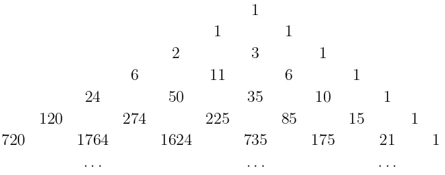
There are n! permutations of n letters. These permutations have various numbers of cycles, from a minimum of one cycle to a maximum of n cycles. For each n, k we introduce the binomial-coefficient-like symbol hnki for the number of permutations of n letters that have exactly k cycles. These are the Stirling cycle numbers. In the literature they are also called the absolute values of the Stirling numbers of the first kind. Thus, for each n we will have P
1
1 1
2 3 1
6 11 6 1
24 50 35 10 1
120 274 225 85 15 1
720 1764 1624 735 175 21 1
. . . .
Figure 4.2: The triangle of Stirling cycle numbers
4.4
East side, west side ... (II)
Fix positive integersn, k. Imagine that all of the permutations ofn letters that have exactly k cycles have been strewn on the sidewalks and streets, all around the town. Now take a walking tour and inspect them as they lie on the ground. If, in a certain permutation, the letter n lives in a cycle all by itself, then move that permutation to the east side of town, and if, on the contrary,n lives in a cycle with at least one other letter, then move it to the west side.
Now instead of one large collection of permutations all over the place, we have two nice neat piles, one on the east side, and the other on the west side of town.
How many permutations are on the east side? These are the ones in which n lives all by itself in a cycle of length 1. How many such permutations are there? Well, since n lives alone, the rest of the permutation must be comprised ofk−1 cycles involving the other n−1 letters. That means that altogether, there are hn−1
k−1
i
permutations that are stacked up on the east side.
How many are on the west side? These are the ones in which n lives in a cycle with other letters. If we remove the letter nfrom the cycle that it lives in, we will be looking at some permutation ofn−1 letters into the same number, k, of cycles.
However, the converse is a bit sticky. If, conversely, we take some permutation of n−1 letters into k cycles, there are many ways in which we might insert the lettern into one of the cycles. In fact, since there are n−1 letters in the permutation, and we can insert the letter n in between any two consecutive letters on any cycle, there are n−1 ways to insert n.
number of permutations ofn−1 letters into k cycles, i.e., it is (n−1)hn−1 k
i .
Therefore the number of all permutations of n letters that have k cycles must be equal tohnk−−11
i
+ (n−1)hn−k1i since every such permutation landed on one side of town or the other.
Theorem 4.1 The Stirling cycle numbers hnki satisfy the Pascal-triangle-like recur-rence
Here is a recursive Maple procedure to calculate the Stirling cycle numbers.
StirCyc:=proc(n,k) options remember;
#Returns the no. of perms of n letters with k cycles if n<1 then RETURN(0)
From the recurrence (4.1) we can easily find a nice formula for the generating function
fn(x) =
and that formula will come in handy when we want to find the average number of cycles that permutations of n letters have.
To find it, multiply both sides of (4.1) by xk and sum over all integers k. On the
left side we will obtainfn(x), the unknown generating function. The second term on
the right will give us (n−1)fn−1(x), so that part is easy.
What about the first term on the right? It is
(Be sure to absorb that footwork before proceeding.) We have found that fn(x) =xfn−1(x) + (n−1)fn−1(x) = (x+n−1)fn−1(x).
Since f1(x) = x (why?), we find successively that f2(x) = x(x+ 1), f3(x) = x(x+
1)(x+2), and so forth. By induction, it is trivial now to establish the following result.
Theorem 4.2 The Stirling cycle numberhnki is the coefficient ofxk in the polynomial
x(x+ 1). . .(x+n−1). That is, we have
and the row of coefficients is identical with the fourth row in the triangle of Fig. 4.2 (do have a look, and check this).
4.6
The average number of cycles
On average, how many cycles does a permutation of nletters have? We use equation (3.2) for the average expressed in terms of the probabilities of each value.
First, what is the probability that a permutation of nletters has exactlyk cycles? Evidently it ispk=
hn
k
i
/n!. Now from equation (3.2) we have that the average number of cycles among permutations ofn letters, let’s call it ¯k(n), is
¯
If you ever have to differentiate a function g(x) which is a product of lots of things, as is the case here, it’s usually better to use the fact that
With g(x) = x(x+ 1). . .(x+n−1), this reads as
If we substitute this in (4.3) we find that ¯
Let’s define the nthharmonic number Hn to be
Hn =
Theorem 4.3 The average number of cycles that permutations of n letters have is the harmonic number Hn.
When n is large, the harmonic number Hn is well approximated by logn, as can be
seen by comparing it with the integral Rn
1 dt
t. So permutations of n letters have an
average of about logn cycles.
4.7
An application
We consider an application of the theory of permutations and their cycles to a simple algorithm for finding the largest member of a set or list.
Suppose {a1, a2, . . . , an} is a given list of n numbers, and we want to find the
largest number in the list. We’ll use the obvious algorithm, namely we will test each ai, in turn, against the current contents of a certain quantity, winner, say. If ai >
winner, then ai will replace winner. Otherwise we just go to the next value of i.
-bigone:=proc(a,n) local winner,i;
# Returns the largest element of a given # array a of length n.
winner:=a[1];
for i from 2 to n do
if a[i]>winner then winner:=a[i] fi; od;
RETURN(winner); end:
We want to know about the complexity of this routine, that is, about the amount of labor that is involved in using it. At first glance this seems totally trivial since we do one pairwise comparison (“if a[i]>winner then ..”) for each i, the thing does about n pairwise comparisons, and that all there is to say, right?
No, there’s more to say. Aside from the pairwise comparisons of size, this algo-rithm does another kind of work: it moves data from one place to another. Every time that a[i] is bigger than winner, the program moves a[i] to winner. How much work is that? It depends. What it depends on is how many times that data movement takes place. In other words, it depends on the number of times that we find an array entry a[i] that is larger than the current occupant of the winner’s circle.
Let’s assume that the array entries are all distinct. Then all that matter are the
relative sizes of the array entries, so we might as well assume that the input array is (the 2nd line of the 2-line form of) a permutation of n letters.
As we read (‘parse’) the values of the permutation from left to right, the number of times the algorithm will have to replace the contents of winner is equal to the number of values of i for which a[i] is larger than all a[j] for j < i. Another way to think about it is that we are interested in the number of times a new world’s record is set, as we read the values of the input permutation. For example, if the input list is
[6,2,4,8,1,9,5,3,10,7]
then 4 world’s records are set, since each of the 4 entries 6,8,9,10 is larger than every entry to its left.
So our question is, what is the average number of outstanding elements that per-mutations of n letters have? Whatever that answer is, it’s also the average amount of work that our algorithm will have to do by moving pieces of data around.
Theorem 4.4 The number of permutations of n letters that have k outstanding ele-ments is equal to the number that have k cycles.
To see why this is so, we will exhibit an explicit 1-1 mapping between these two flavors of permutations.
First, given a permutation of n letters with k cycles, say σ, do the following. 1. Standardizeσ by presenting the cycles in such a way that the largest element of
each cycle appears first in that cycle, and the sequence of cycles ofσis arranged so that, from left to right, the sequence of largest elements within each cycle increases.
2. Then drop all of the parentheses that appear in the cycle presentation of σ. 3. Interpret the result as the second line of the two line form of a certain
permu-tationf(σ). This latter permutation has exactly k outstanding elements. Conversely, if we are given the second line of the two line form of f(σ), we can recover σ uniquely as follows.
1. Place a left parenthesis at the extreme left of the given line.
2. Read the line from left to right, and each time an element xis encountered that is larger than every element to its left, put a right parenthesis and an opening left parenthesis immediately to the left ofx.
3. Place a right parenthesis at the extreme right of the given line.
4. Interpret the result as the cycle form of some permutation σ. That permutation
will have exactly k cycles. ✷
Conversely, if we are given f(σ) = 4623751, we insert parentheses as instructed to get (4)(623)(751), which is the cycle form of a permutationσ with three cycles.
It follows from the theorem that the average number of outstanding elements of permutations ofn letters is the same as the average number of cycles, namely, exactly Hn, and approximately logn.
Therefore, in the course of finding the largest element of a given array, it will happen about logn times, on the average, that we will move some data from the array to winner.
4.8
Making lists and random choices of permutations and
their cycles
Again, the counting arguments in this section will immediately suggest ways of making lists of permutations with given numbers of cycles and of making random choices of them.
Suppose n, k are given. To make a list of all permutations of n letters that have k cycles, let’s list those in which n lives in a cycle by itself first, and then all of the others second. Suppose L(n, k) denotes this list of permutations.
To list those in whichnlives alone, we take the full list L(n−1, k−1), and we glue onto each permutation on that list a new cycle that contains only the lettern. To list those in whichnlives in a cycle with other letters, we take the full listL(n−1, k), and for each permutation on that list we constructn−1 new permutations by insertingn succesively into the “cracks” between consecutive elements around each of its cycles. Let’s make the list L(4,2). First take L(3,1), which consists of the two permu-tations (123) and (132), in cycle form. We glue onto these two a new cycle that contains only the letter 4, to obtain the two east side permutations (123)(4) and (132)(4). Now take the list L(3,2), which consists of the three permutations (1)(23), (2)(13), and (3)(12), and insert the new letter 4 into each position between two con-secutive letters on each cycle. This yields the nine west side permutations (41)(23), (1)(423), (1)(243) and (42)(13), (2)(413), (2)(143) and (43)(12), (3)(412), (3)(142). The desired list L(4,2) consists of the two east side followed by the nine west side permutations that we have just constructed.
Here is a Maple procedure6
to make a list of all n-permutations with k cycles. Remarkably, it turns out to be nicer to implement this using the 2-line form of the permutation rather than the cycle form.
6
eastop:=(y,j)->[op(y),j]:
westop:=(y,j)->[op(subsop(j=1+nops(y),y)),y[j]]: ListKPerms:=proc(n,k)
local east,west,out,j ; options remember;
#Lists, in 2-line form, the perms of n letters, k cycles if n<1 or k<1 or k>n then RETURN([])
else if n=1 then RETURN([[1]])
else
east:=ListKPerms(n-1,k-1);west:=ListKPerms(n-1,k); out:=map(eastop,east,n);
for j from 1 to n-1 do
out:=[op(out),op(map(westop,west,j))] od; RETURN(out);fi;fi;
end:
To run this program, we might callListKPerms(4,2); and the output would then be as follows:
[[3,1,2,4],[2,3,1,4],[4,1,3,2],[4,2,1,3],[4,3,2,1],[2,4,3,1],
[3,4,1,2],[1,4,2,3],[2,1,4,3],[3,2,4,1],[1,3,4,2]] (4.4) Thus the output shows the eleven permutations of four letters that have two cycles. Notice that each permutation is displayed with the second line of its 2-line form, and not in its cycle form. Thus, the first output permutation, which is shown as [3, 1, 2, 4], is the permutation f for which f(1) = 3, f(2) = 1, f(3) = 2, f(4) = 4, which indeed has two cycles.
How do we choose a permutation of n letters and k cycles uniformly at random? First we decide whether we are going to choose an east side or a west side permu-tation. How to do that? Well, the probability of choosing an east side permutation is obviously p = hnk−−11i/hnki. So calculate the number p, and then choose a random real number ξ in the range (0,1). If ξ < p then the output will be an east side permutation, and otherwise it will be a west side permutation.
k cycles. In this permutation there are n−1 cracks between consecutive letters on cycles. Choose one of these cracks uar and insert the new letter n into the chosen crack. All finished.
Here is a Maple procedure7
that will do the random selection. Again, the proce-dure presents the output as the sequence of values of the permutation chosen, rather than in cycle form.
RandKPerms:=proc(n,k) local rno,r,east,west,rn ;
#Returns a random perm of n letters, k cycles, in 2-line form if n=1 then
if k<>1 then RETURN([]) else RETURN([1]) fi; else
4.9
Ranking permutations by cycles
What is the rank of the permutation τ := (16)(382)(45)(7) (cycle form) of 8 letters with 4 cycles in the list of all such permutations? Recall our scheme for listing these permutations. First in the list are those in which the highest letter, in this case 8, is a fixed point of the permutation. In τ, 8 is not a fixed point. Thus all of the h73
i permutations in which 8 is a fixed point have lower rank than τ.
After those in the list come the h74
i
permutations σ for which σ(1) = 8, then the h7
plus the rank of the deleted permutation τ′ := (16)(32)(45)(7) in the list of all permutations of 7 letters and 4 cycles. This
leads to the following Maple program for ranking permutations by cycles. It uses the program StirCyc, of page 26 above.
7
RankPermsCycles:=proc(ss,n,k) local jj,tt;
if k=n or k=0 then RETURN(0) elif ss[n]=n
then RETURN(RankPermsCycles(subsop(n=NULL,ss),n-1,k-1)) else
member(n,ss,jj); tt:=ss;
tt[jj]:=tt[n];
tt:=[op(1..n-1,tt)];
RETURN(RankPermsCycles(tt,n-1,k)+(jj-1)*StirCyc(n-1,k)+StirCyc(n-1,k-1)) fi:
end:
4.10
Exercises
1. Exhibit a permutation of n letters, other than the identity permutation, whose “square” is equal to the identity. That is, find a permutation f such that f◦f is equal to the identity. Such a permutation is called an involution. What do the cycles of an involution look like?
2. Suppose that a certain permutationf, ofn letters, hasνi cycles of lengthi, for
each i= 1,2, . . .. Then how many cycles of each length does f◦f have? 3. The order of a permutation f in the group Sn of all permutations of n letters
is the least positive integer k such that fk is the identity permutation. Express
the order of a permutation f in terms of the lengths of its cycles. 4. Describe the cycles of f−1
in terms of those of f.
5. How many permutations of n letters have exactly two cycles? That is, find a simple formula for hn2
i .
6. Fix positive integers n and j, with j ≤ n. Choose a random permutation of n letters. What is the probability that the element n lives in a cycle of length j? (Note that the answer depends remarkably little onj.)
4.11
Maple Programming Exercises
is the list of values off ◦g.
2. Write a Maple procedure InvertIt(f) whose input is the list of values of a permutation f, and whose output is the list forf−1
.
3. Write a Maple procedure MaxOrder(n) that will use the result of exercise 3 above to find the largest possible order that a permutation of n letters can have. Run this program for n = 2,3, . . .up to as large a value of n as you can manage, and tabulate the largest possible orders as a function ofn.
4. Write a Maple program which, for given n, will print a list of the Stirling cycle numbers of order n, by using the following method. Take the generating polynomial (4.2), expand it, and print out its coefficient list. Use the Maple instructions expand, product, and coeffs.
5. Same as the previous problem, except instead of using the expand instruction, use the Maple series instruction. For a technical matter, you will need the instructionconvert(...,polynom)in order to convert the output of theseries command to the form of a polynomial, so that its coeffs can be extracted. 6. Write a Maple program RandTestthat will generate 1000 random real numbers
x in the range 0¡x¡1 (do not print these individual numbers), and which will output a table showing how many of those 1000 lay in the interval (0,.1), how many were in (.1,.2), ..., how many were in (.9, 1.0), Use the Maple instruction rand(). Do the results look random?
7. Write a Maple procedureRandPerm which, given a positive integernwill output a randomly chosen permutation ofnletters in the form of the second line of the 2-line form of the output permutation.
8. Write a procedure CountCycles(f) that will take as input a list of length n that is the second line of the 2-line form of a permutation and will output the number of cycles that the input permutation has.
5
Set partitions
5.1
What set partitions are
A partition of a set S is a collection A1, . . . , Ak of nonempty subsets of S for which
(i) For all 1≤i < j ≤k, Ai∩Aj =∅, and
(ii) S =A1∪A2∪. . .∪Ak.
The sets Ai are the classes of the partition.
We can write a particular set partition by using braces, each pair of which contains the elements of one of the classes Ai. Thus
{1,4,5},{2},{3,6}
is one way to partition the set{1,2,3,4,5,6}into three classes. For computer work it is often better to represent a set partition by means of itsclass vector. For a partition of{1,2, . . . , n}intokclasses, the class vector is of length n, and for eachi= 1, . . . , n, itsith entry is the class to whichibelongs. The class vector of the partition displayed above, for instance, is (1,2,3,1,1,3).
5.2
Counting set partitions by classes
The number of partitions of a set ofn elements intok classes is called theStirling set number, and is denoted bynn
k
o
. It is also called the Stirling number of the second kind. If we make a triangle which contains, in its nth row, the numbers nn1
o ,nn2
o
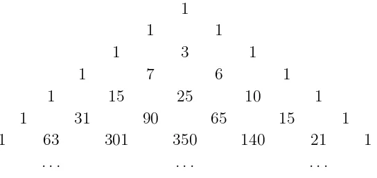
, . . . ,nnno, for each n = 1,2,3, . . ., then we will have the Pascal-like triangle that these set numbers occupy. It begins as shown in Fig. 5.3.
Look at the sums of the rows in this Stirling triangle. These are the numbers 1,2,5,15,52, . . ., and they are called the Bell numbers. The Bell number b(n) is the number of partitions of a set of n elements. So b(4) = 15 means that there are 15 ways to partition a set of 4 elements. Can you write them all out?
Let’s take some particular number in this array and try to visualize what it counts. Like the 6 that appears in the (n, k) = (4,3) position in the array. It says that a set of 4 things can be partitioned into 3 classes in exactly 6 ways. These 6 ways are
1
1 1
1 3 1
1 7 6 1
1 15 25 10 1
1 31 90 65 15 1
1 63 301 350 140 21 1
. . . .
Figure 5.3: The triangle of Stirling set numbers
5.3
East side, west side ... (III)
Fix positive integers n, k. Imagine that all of the partitions ofn letters into exactly k classes have been strewn on the sidewalks and streets, all around the town.
Now take a walking tour and inspect them as they lie on the ground. If, in a certain set partition, the letter n lives in a class all by itself, then move that set partition to the east side of town, and if, on the contrary, n lives in a class with at least one other letter, then move it to the west side.
Now instead of one large collection of set partitions all over the place, we have two nice neat piles, one on the east side, and the other on the west side of town.
How many set partitions are on the east side? These are the ones in which n lives all by itself in a class of size 1. How many such set partitions are there? Well, sincen lives alone, the rest of the partition must be comprised of k−1 classes involving the other n−1 letters. That means that altogether, there are nn−1
k−1
o
set partitions that are stacked up on the east side.
How many are on the west side? These are the ones in which n lives in a class with other letters. If we remove the lettern from the class that it lives in, we will be looking at some partition of n−1 letters into the same number, k, of classes.
However, the converse is a bit sticky. If, conversely, we take some partition of n−1 letters intok classes, there are many ways in which we might insert the lettern into one of the classes. In fact, since there arek classes in the partition, and we can insert the letter n into any class, there are k ways to insert n.
Therefore the number of all set partitions of n letters that have k classes must be equal tonnk−−11
o
+knn−k1o since every such partition landed on one side of town or the other.
Theorem 5.1 The Stirling set numbers nnko satisfy the Pascal-triangle-like recur-rence
It is important to observe that numbers that are defined recursively can be calcu-lated recursively, i.e., with a computer program that calls itself. This can be done only in a recursion-capable computer language. In Maple, a procedure that will calculate nn
#Returns the Stirling number of the 2nd kind if n<1 then RETURN(0)
If we look for the generating function of the Stirling set numbers nnko, we might be tempted to multiply both sides of (5.1) byxk and sum over all integerk, as we did in
the case of the cycle numbers. Here, though, we would be doomed to failure, because of the appearance of the “k” on the right side of (5.1), which would interfere with that operation mightily.
Instead, let’s define the generating functions fk(x) =Pn
nn
k
o
xn, and we will
suc-ceed in finding them explicitly. To do that, multiply (5.1) on both sides byxnand sum
onn. The result is thatfk(x) =xfk−1(x) +kxfk(x), i.e.,fk(x) = (x/(1−kx))fk−1(x).
Theorem 5.2 The Stirling set number nnko is the coefficient of xn in the generating
function xk/((1−x)(1−2x)(1−3x). . .(1−kx)). That is, we have
X
n≥0
( n k )
xn = x
k
(1−x)(1−2x)(1−3x). . .(1−kx) (k = 1,2,3, . . .) (5.2)
5.5
An application
Suppose that there are d different kinds of coupons, and that we want to collect at least one specimen of each kind. We embark on a series of trials, in each of which we choose, uniformly at random, one of the coupons and add it to our collection. What is the probability that at thenth trial we find, for the first time, that we have at least one specimen of all of thed kinds of coupons?
Let p(n, d) denote the required answer.
If at the nth trial we have a complete collection for the first time, then suppose we happened to have chosen couponi at thatnth trial. Theni was the only missing coupon from the results of the firstn−1 trials. That means that the first n−1 trials had at least one specimen of each of the coupons 1,2, . . . , i−1, i+ 1, . . . d, and that the missing type i was then chosen.
For each j = 1, . . . , n, let a[j] denote the number of the coupon that was drawn on thejth trial. For n= 10, d= 4, i= 3, for instance, the array (a[1], a[2], . . . , a[10]) might look like
(1,4,4,1,2,4,4,2,1,3).
We observe that this array a describes (‘encodes’) a certain set partition of the set
{1,2, . . . , n−1} into d−1 classes. Indeed, the class to which the letter j belongs is a[j]. The example array above describes a partition of the set {1,2, . . . ,9} into 3 classes, namely the partition {1,4,9},{5,8},{2,3,6,7}.
But there’s a little difference that’s important. The classes of the partition are
ordered. That is, the partition {1,4,9},{5,8},{2,3,6,7} is counted as a different partition from the partition {5,8},{2,3,6,7},{1,4,9}, for example. That’s because the first of these two partitions comes from the array (1,4,4,1,2,4,4,2,1,3), as we saw, while the second comes from the array (4,2,2,4,1,2,2,1,4,3). The number of partitions with ordered classes that correspond to a single partition into k classes is k!, since there are that many ways to rearrange the classes.
Thus we can describe the sequence of trials of a coupon collector who succeeded on the nth trial in getting a complete collection of coupons, by giving the vector a
can be done in (d−1)!nn−1 d−1
o
ways for each choice of the index i that completes the sequence, for a total of d!nnd−−11
o
ways altogether.
To return to the probability that n trials will be needed, that is the number of possible vectorsathat correspond ton trials, divided by the total number of possible outcomes on n trials, which is dn, that is, the probability that exactly n trials are
needed is
The probability generating function is
f(x) =X
If we refer to (5.2) the above can be rewritten as
f(x) = X
We note in passing thatf(1) = 1, as must be true for probability generating functions.
Theorem 5.3 The probability that exactlyn trials will be needed to complete a collec-tion of d different coupons is the coefficient of xn in the power series for the function
= d+
d−1
X
j=1
j
d−j =d+
d−1
X
j=1
(j−d) +d d−j
= d−(d−1) +d
d−1
X
j=1
1
d−j = 1 +d(Hd− 1
d) =dHd
Theorem 5.4 The average number of trials that are needed to complete a collection of d kinds of coupons is dHd, where Hd is the harmonic number.
5.6
Making lists and random choices of set partitions
To make a list L(n, k) of all partitions of {1,2, . . . , n} into k classes, we do the following. Take the list L(n −1, k−1), and to each partition on that list adjoin a new class consisting solely of the letter n. That will list the portion of L(n, k) that comes from the east side. Next, take the list L(n−1, k), and for each partition Π on that list create k new partitions, namely those that are obtained by inserting the letter n as a new member of each of the k classes, in turn, of Π.
A good data structure for representing a set partition in a computer is the class vector of the partition. The class vector of a partition of the set {1,2, . . . , n} into k classes is the n-vector (a1, a2, . . . , an) in which for each i, ai is the class to which
i belongs. Thus the partition (1,7)(2,3,5)(4,6) of {1,2, . . . ,7} into three classes is represented by the class vector (1,2,2,3,2,3,1).
To adjoin a new class consisting solely of the letter n, we take the class vector and adjoin one new entry to it, namely the entry an=k. To insert n into one of the
already existing k classes, we take the class vector and adjoin one new entry to it, namely the entry an =i, if i is the index of the class into which we are inserting the
letter n.
A Maple procedure8
for making a list of all partitions of{1,2, . . . , n}intok classes is as follows.
8
EWop:=(y,m)->[op(y),m]: ListSetPtns:=proc(n,k)
local east,west,i,out ; options remember;
#Lists all partitions of the set 1,..,n into k classes #Output array[i] is the class to which i belongs. if n=1 then
if k<>1 then RETURN([]) else RETURN([[1]]) fi: else
east:=ListSetPtns(n-1,k-1): west:=ListSetPtns(n-1,k): out:=map(EWop,east,k);
for i from 1 to k do out:=[op(out),op(map(EWop,west,i))] od; RETURN(out);
fi: end:
A procedure that will select a partition of the set{1,2, . . . , n}withkclasses uar is also easy to do recursively. With probabilitynnk−−11
o
/nnkowe will choose uar a partition of{1, . . . , n−1}intok−1 classes and then insert the lettern as a new singleton class. With probability 1−nn−1
k−1
o
/nnko, we will choose uar a partition of{1, . . . , n−1}into k classes and then insert the letter n into a randomly chosen one of those k classes. The Maple program9
follows.
RandSetPtns:=proc(n,k) local rno,class ;
#Returns a random partition of 1..n into k classes if n=1 then
if k<>1 then RETURN([]) else RETURN([1]) fi; else
rno:=10^(-12)*rand();# Choose a random real number in (0,1) if rno<StirSet(n-1,k-1)/StirSet(n,k)
then #we go to the east side
RETURN([op(RandSetPtns(n-1,k-1)),k]) else #we go to the west side
class:=rand(1..k);
RETURN([op(RandSetPtns(n-1,k)),class()]) fi;
fi; end:
9
5.7
Ranking set partitions
What is the rank of the partition Π :={1,4}{2,7,8}{3}{5,6}of the set{1,2, . . . ,8}
into 4 classes in the list of all partitions of that set into 4 classes?
Our list of partitions puts those set partitions in which the highest letternlives in a singleton class first. Following those are the partitions in which n lives, not alone, in class 1, then those in which n is, not alone, in class 2, etc., where the classes are numbered in order of their smallest element. For this example partition Π, 8 is not in a singleton class, so it is preceded in the list by all of the n7
3
o
partitions in which 8 does live in a singleton class. Further, 8 does not live in the first class of Π, so Π is also preceded by all n74
o
partitions that are obtained by inserting 8 into the first
class of some partition of 7 letters into 4 classes.
Thus, if Π′ denotes the partition obtained from Π by deleting 8, then
rank(Π) = (
7 3 )
+ (
7 4 )
+ rank(Π′
),
which is the idea of the recursive algorithm. The full Maple program for ranking set partitions is as follows.
5.8
Exercises
1. Find a simple formula for the number of partitions of a set of n elements into 2 classes, i.e., for the Stirling set number nn2o.
2. In how many partitions of a set ofn elements does the element n live in a class of size j? Express your answer in terms of the Bell numbers.
6
Integer partitions
6.1
What they are
A partition of an integer n is a representation of n as a sum of positive integers, the order of the latter being immaterial. The partitions of 5 are 5, 4 + 1, 3 + 2, 3 + 1 + 1, 2 + 2 + 1, 2 + 1 + 1 + 1, and 1 + 1 + 1 + 1 + 1, so we can partition the integer 5 in 7 ways. If p(n) denotes the number of partitions of the integern, then the sequence of values of p(n), for n= 0,1,2, . . ., begins as
{1,1,2,3,5,7,11,15,22,30,42,56,77,101,135,176, . . .}.
Generically, we will write a partition as n =a1+a2 +. . .+ar, where a1 ≥ a2 ≥
. . .≥ar ≥1. The numbers ai(i = 1, . . . , r) are the parts of the partition. So we will
standardize by presenting a partition with its parts in nonascending order.
Let p(n, k) denote the number of partitions of the integer n whose largest part is k. For example, p(4,2) = 2 since there are two partitions of 4 whose largest part is 2, viz., 4 = 2 + 2 and 4 = 2 + 1 + 1. The table of values ofp(n, k), with rows labeled by n = 1,2, . . ., looks like this.
1
1 1
1 1 1
1 2 1 1
1 2 2 1 1
1 3 3 2 1 1
1 3 4 3 2 1 1
The suspense is geting unbearable. Could it be that we have yet another east side-west side situation developing here?