Minimum Constructive Back Propagation Neural Network Based on Fuzzy Logic for Pattern Recognition of Electronic Nose System

Minimum Constructive Back Propagation Neural

Network Based on Fuzzy Logic for Pattern

Recognition of Electronic Nose System

Radi, Muhammad Rivai, and Mauridhi Hery Purnomo1

AbstractConstructive Back Propagation Neural Network (CBPNN) is a kind of back propagation neural network trained with constructive algorithm. Training of CBPNN is mainly conducted by developing the network’s architecture which commonly done by adding a number of new neuron units on learning process. Training of the network usually implements fixed method to develop its structure gradually by adding new units constantly. Although this method is simple and able to create an adaptive network for data pattern complexity, but it is wasteful and inefficient for computing. New unit addition affects directly to the computational load of training, speed of convergence, and structure of the final neural network. While increases training load significantly, excessive addition of units also tends to generate a large size of final network. Moreover, addition pattern with small unit number tends to drop off the adaptability of the network and extends time of training. Therefore, there is important to design an adaptive structure development pattern for CBPNN in order to minimize computing load of training. This study proposes Fuzzy Logic (FL) algorithm to manage and develop structure of CBPNN. FL method was implemented on two models of CBPNN, i.e. designed with one and two hidden layers, used to recognize aroma patterns on an electronic nose system. The results showed that this method is effective to be applied due to its capability to minimize time of training, to reduce load of computational learning, and generate small size of network.

KeywordsCBPNN, structure development pattern, fuzzy logic, effective

AbstrakConstructive Back Propagation Neural Network (CBPNN) adalah jaring saraf perambatan balik galat yang dilatih dengan algoritma konstruktif. Pelatihan CBPNN pada dasarnya dilakukan melalui metode pengembangan arsitektur jaring yang biasanya dilakukan dengan menambahkan sejumlah neuron baru pada lapis tersembunyi pada proses pelatihannya. Pelatihan jaring saraf ini dapat dilakukan dengan metode fixed, yaitu metode pengembangan struktur jaring dengan pola penambahan sejumlah neuron konstan secara bertahap. Meskipun cara ini mudah dilakukan dan telah mampu membangun struktur jaring yang adaptif terhadap kempleksitas data pelatihan, namun dari sisi komputasi dipandang kurang efisien. Penambahan neuron baru secara langsung berdampak terhadap beban komputasi pelatihan, kecepatan konvergensi, dan struktur jaring saraf yang terbentuk. Selain memberatkan beban komputasi, penambahan neuron yang terlalu banyak cenderung menghasilkan struktur jaring akhir yang besar. Di lain pihak, pola penambahan dengan sedikit neuron dapat menurunkan kemampuan adaptasi jaring saraf dan cenderung menambah waktu pelatihan. Oleh karena itu, pola pengembangan struktur jaring CBPNN yang adaptif perlu didesain untuk menurunkan beban komputasi pelatihan. Penelitian ini mengusulkan algoritma Fuzzy Logic (FL) untuk mengadaptifkan pengembangan struktur jaring CBPNN. Metode FL ini diterapkan pada pelatihan CBPNN dengan dua struktur, yaitu CBPNN dengan satu lapisan tersembunyi dan CBPNN dengan dua lapisan tersembunyi. Hasil penelitian menunjukan bahwa metode ini cukup efektif untuk diterapkan karena mampu meminimumkan waktu pelatihan, mengurangi beban komputasi dan menghasilkan struktur jaring saraf akhir yang lebih kecil.

Kata KunciCBPNN, pola pengembangan struktur, logika fuzzy, efektif

I.INTRODUCTION4

lectronic nose system is artificial olfaction technology, works as a representative of human olfactory system, usually used to analyze gaseous mixtures, discriminate different mixtures, or quantify the concentration of gas component. This instrument consists of four main parts, namely an odor sampling system, odor sensitive receptor, electronic circuitry, and data analysis software. Part of odor receptor usually implements a number of gas sensors arranged in an array form. While a pattern recognition software is commonly used to analyze the data [1]. Beside sensors, performance of the electronic nose system is determined by pattern recognition system. One of the pattern recognition algorithm broadly used in electronic nose systems is Artificial Neural Network (ANN). Researches on electronic nose system by using ANN as pattern

Radi, Muhammad Rivai, and Mauridhi Hery Purnomo are with Department of Electrical Engineering, FTI, Institut Teknologi Sepuluh

Nopember, Surabaya, 60111, Indonesia. Email:

radi10@mhs.ee.its.ac.id.

recognition algorithms for product quality have been conducted, such as applied to identify the quality of tea and spoiled beef [2-3].

ANN algorithm has been developed and mostly applied in many disciplines especially those related to the artificial intelligence systems. ANN is very helpful in the field of control and pattern recognition systems. Implementation of ANN increased significantly in recent decades, mainly supported by the development of pattern recognition research for various object studies. One model of ANN usually used as pattern recognition is Multi Layer Perceptron (MLP). MLP network can be trained with error back propagation method. Hence, this network is often popular with Back Propagation Neural Network (BPNN) [4]. Study showed that compared to other networks, BPNN has better performance [5].

BPNN has great ability to identify and recognize data patterns. Performance of the network is very dependent on the network architecture. The solution quality found by general BPNN depends strongly on the network size used. Size of network also determines learning process and its ability to recognize a given data pattern. Small structure of BPNN has limited capability to classify and

identify complex patterns. Otherwise, BPNN with larger structure has better performance to recognize difficult patterns accurately [6-8]. On the other hand, large-sized of BPNN is more difficult to be trained than the small one. Choosing large size of BPNNs in one case often does not improve their performance and tends to aggravate the computational burden of training. Moreover, large size neural network commonly contains of noise, which cause the network lose its ability to recognize patterns [7-8]. Therefore, properly network has to be designed carefully.

Application of small BPNN provides many advantages. Small BPNN can be easily trained with a light computational load. Besides, this network is also programmable. Implementation of this network requires only a minimum space of memory. Today, technology enables to design a portable electronic nose by applying microprocessor such as microcontroller or FPGA. In this system, application of small neural network is desirable. Therefore, designing minimum size of ANN is required. Researchers still investigate and review some algorithms in order to design minimum neural networks, such as finding minimum network by using pruning methods for business intelligent applications [9].

There are three methods commonly used to design neural network correspond to the patterns which want to be classified [6]. First is trial and error method. This method is conducted by training various sizes of neural network for a training data set, and then selects an appropriate neural network. Beside difficult to be implemented, this method needs experiences. The second method is pruning algorithm. Firstly, we train large size network. During training, the network size is reduced by eliminating some neurons, which have less contribution to the network outputs. Elimination of unnecessary neuron is done continuously in order to obtain an appropriate neural network. The last is constructive method. Training of the neural network is started with simple architecture. Adding new unit progressively is required to develop the initial network. Training is finished when the network was able to classify the data pattern. Other methods are developed by combining some of these methods.

Constructive method has advantages compared to other methods [4, 6]. Constructive method applied on neural network is used to modify its previous structure in order to get a proper neural network. Constructive algorithm tries to find suitable network from very simple architecture, so this algorithm is easy to be computed. Besides, this method also tends to generate smaller network. In addition, it is also consistent to the provisions of CASA (Continuous Automation Structure Adaptation) which commonly used as standard of adaptive neural network.

BPNN trained with constructive method is known as Constructive Back Propagation Neural Network (CBPNN). Training of CBPNN can be characterized by developing structure of the network gradually in order to create adaptive algorithm for various complexity of training data patterns. Before trained, the neural network is initiated by a simple structure. This initial network is trained to recognize a given training data. If the first network fails to recognize the patterns, developing structure has to be conducted by adding new neurons in

the hidden layer. Adding unit is approved continuously until the neural network produce accurate results on patterns outside its training set.

Pattern of structures development is the focus on training of CBPNN. Pattern by adding new unit constantly, which in this paper referred to fixed method, is structure development pattern that widely implemented to train of general CBPNN. In this method, number of new units added at each step of training should be managed fixedly. Although the training pattern can be implemented easily and creates adaptive CBPNN for the data patterns complexity, but it is wasteful and inefficient computing. Adding size of network will affect to the computational load of learning, speed of convergence, and structure of the final network. Change of structure due to new unit added tends to enlarge load of computational running. Adding new unit means increasing neuron number and network connection simultaneously. Lot of neurons needs hard effort to be computed. Besides, too many connections must be modified concurrently. In addition, excessive addition pattern while increasing computational load also tends to produce large-sized of final network. Furthermore, addition pattern by too small new unit number will reduce the network adaptability and extend time to learn. Therefore, there is important to design adaptive structure development pattern for CBPNN in order to minimize load of training process.

The aim of this study is to implement Fuzzy Logic algorithm (FL) in training of CBPNN. This algorithm will be used to modify structure development pattern of CBPNN. Modifying structure development is desired to minimize effort and to streamline training process of the network. We expect that this method is powerful to be implemented on training of CBPNN.

II.METHOD

A. Basic Training of CBPNN

Learning process is finished when the network converges at the specified error threshold.

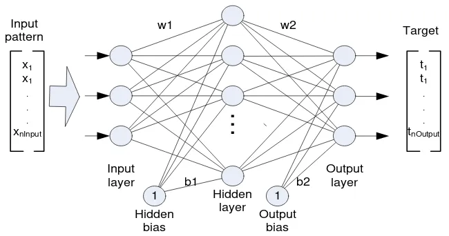
Training network with back propagation involves three steps, they are: step to feed-forward all input patterns, step to calculate and back propagate the associated error, and step to modify connection weight of the network [9]. Structure of one hidden layer of BPNN is illustrated on Figure 1. This network consists of n input units of input layer, n hidden neurons of hidden layer, n output neurons of output layer, hidden bias, and output bias. w1 is connection weights between input layer and hidden layer, b1 is connection weights of hidden bias and hidden layer, w2 is connection weight of hidden layer and output layer, and b2 represents connection weight between output bias and output layer.

Before training is started, we ought to prepare a training data set. This data consists of n data pairs of input data pattern xi(i = 1, 2, 3, … n input) and target tj

(j = 1, 2, …n output). These Data Patterns prepared (DP) can be formulated as follows:

)} t , (x , ), t , (x ), t , {(x

DP 1 1 2 2  nDat a nDat a (1)

w1, b1, w2, b2 are firstly initiated by randomize function.

Detail of these steps can be explained as follow: 1. Step to feed-forward the input patterns

This step is also popular with forward step. This step calculates all output signals of the network. Each pair of the training data is used to train the network. The first pair of the data that consist of n input data are used as first input pattern of the neural network. In the input layer, the data is forwarded to all hidden neurons with their related connection weight w1. Each hidden unit (Vj, j = 1, .. n hidden) counts all input signals from the previous layer and connection weight of the bias (b1). Mathematically, it can be formulated as follows:



    nInput i j i i j

j b x w

Vin

1

, 1

1 (2)

All neurons in the hidden layer will issue output signals that appropriate to their activation function (f). Signals of all hidden unit neurons can be written with the following formula:

)

(

_j

j

f

Vin

V



(3)

Then, output signals of the hidden layer are forwarded to all units of the output layer after multiplied with suitable connection weights. Each output unit of the network sums weighted signal of the previous layer and its bias. Output neurons generate output signals (Yk, k = 1, 2, ... n output) based on their activation function, which can be formulated as follows:

)

(

2

2

1 , k k nHidden j k j j k k

Yin

f

Y

w

V

b

Yin











 (4)

2. Step to calculate and back propagate the associated error

This step is frequently called with backward step. This step counts error of the network and propagates the error to all connections of the network. Each output neuron is going to receive target pattern tk accordance with the

training input patterns. Difference between the network outputs and the target is defined as error (ek) of the

network. This error is calculated by the following equation:

k k

k

t

Y

e





(5)

Means Square Error (MSE) of the network can be formulated from the errors with the equation as follow:









   

 nOut put

1 k 2 k k nOut put 1 k 2

k t Y

2 1 e 2 1 MSE (6)

After that, this MSE has to be minimized by gradient descent procedure. This method is conducted by back propagating the error started from the output to the input layer. It is used to modify the overall network connections. Weight corrections of the network can be calculated from the derivative of the MSE for the connection weights which are going to be modified. Weight correction of w2 (Δw2) can be determined with the following equation:

j k k k j k j k k k j k j V Yin f e w w Yin Yin MSE w MSE w                 ) ( ' 2 2 2 2 , , , ,    ₍₇₎

where µ is learning rate parameter. While the weight correction of b2 (Δb2) is determined by the following formula: ) ( ' 2 2 2 2 k k k k k k k k Yin f e b b Yin Yin MSE b MSE b                  (8)

Weight correction of w1 (Δw1) is calculated with the following equation: i j k j k k j i j i j j j j k k j i j i x Vin f w Yin f e w w Vin Vin V V Yin Yin MSE w MSE w                        ) ( ' 2 ) ( ' 1 1 1 1 , , , , ,    (9)

Then, equation 10 is used to calculate weight correction of b1 (Δb1).

) ( ' 2 ) ( ' 1 1 1 1

,k j

j k k j j j j j j k k j j Vin f w Yin f e b b Vin Vin V V Yin Yin MSE b MSE b                          ₍₁₀₎

3. Step to modify connection weight of the network If the network is trained with momentum constant (⍺), weight connection of the network (w1, w2, b1, and b2) can be modified with the following equation:

) ( 2 ) ( 2 ) ( 2 ) ( 2 ) ( 2 ) ( 2 ) ( 2 ) ( 2 ) ( 1 ) ( 1 ) ( 1 ) ( 1 ) ( 1 ) ( 1 ) ( 1 ) ( 1 , , , , , , , , old b new b old b new b old w new w old w new w old b new b old b new b old w new w old w new w k k k k k j k j k j k j j j j j j i j i j i j i                         (11)

Training process is continued until the network is able to recognize the training data pattern, which can be indicated by its ability to convergence at a specified error threshold. Training of BPNN with some hidden layers can be adopted from the previous training algorithm.

Training of CBPNN is conducted with error back propagation algorithm as same as learning process of BPNN. Constructive algorithm is added to modify structure of the network. Principally, training algorithm of general CBPNN can be described into 4 steps, as follows:

a. Initialization step, the phase of initial network configuration. Initial network is constructed without hidden units. The weight of this configuration is updated by error back propagation to minimize the MSE

unit and connecting the new hidden unit to the output units of the network. All connection weights are firstly initialized with random function.

c. Training of new network. After adding new units, the new network is trained by error back propagation to modify connection weight of the network in order to minimize the new MSE. Correcting weight can be done by modifying all network connections or only limited to the new connection added.

d. Convergence test, that is by checking the network output. When the network yields an acceptable solution, then stop the training, otherwise return to step 2.

Adding few hidden units can simultaneously accelerate the formation of the neural network. Besides that, this way tends to minimize the output error faster than training of some units independently [4].

Constructive method effects on the number of hidden unit neuron. The number is modified by pattern of structure development. Constructive method modifies size of the network structure automatically. Hence, learning equation of CBPNN can be rewritten as follows:



    nInput i j i i j

j b x w

Vin 1 , 1 1 (12)



   

 nHiddenNU

j

k j j k

k b V w

Yin 1 , 2 2 (13) j k k k

j

e

f

Yin

V

w











2

_,



'

(

)

(14)

i j k j k k j

i

e

f

Yin

w

f

Vin

x

w















1

_,



'

(

)

2

_,

'

(

)

(15)

)

('

2

)

('

1

_j

e

_k

f

Yin

_k

w

_j,k

f

Vin

_j

b















(16)

where NU is number of new unit and j is used to represent adaptive variable. NU is set constantly on fixed method and is going to be modified by FL method. Then, the new network weight can be determined as follow:

) ( 2 ) ( 2 ) ( 2 ) ( 2 ) ( 2 ) ( 2 ) ( 2 ) ( 2 ) ( 1 ) ( 1 ) ( 1 ) ( 1 ) ( 1 ) ( 1 ) ( 1 ) ( 1 , , , , , , , , old b new b old b new b old w new w old w new w old b new b old b new b old w new w old w new w k k k k k j k j k j k j j j j j j i j i j i j i                         (17)

B. Implementation of Fuzzy Logic on Training Of CBPNN

CBPNN is firstly initiated with simplest structure, commonly without hidden unit. In this study, we design one neuron in the hidden layer for the first arrangement. This initial configuration is trained to recognize data pattern provided at limited iteration. If the network fails to recognize the data set, some neurons are added to the hidden layer. Then the new network architecture is trained with the previous pattern. Training process is continued until we get suitable network for the training data set. Training method by modifying structure is typical algorithm of CBPNN.

As already discussed, changing of network structure effects to the computing process. The number of new units added has to be tuned carefully to simplify

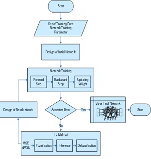
computational process of training. Fast and slow structure changes will be not effective in learning process [6]. In order to minimize training process, structure development pattern has to be managed. Number of new units ought to be adjusted based on the error value at that step. If the network issue signal with big error then a number of hidden units must be added, but if the error is small means that the network has been closely to the expected structure. In this condition, the network only needs addition time to convergence and even does not require new neurons. On the other cases, rapid dropping off error indicates that the network is possible to recognize the training data set. Based on the previous consideration, number of new units should be modified automatically and called with adaptive structure development pattern. FL algorithm is used to the algorithm. Implementation of FL on training of CBPNN can be presented on Figure 2.

FL algorithm is designed by two inputs. Both inputs are formulated on fuzzy rules to generate FL output that represents new unit number should be added. Fuzzy logic thinking involves three processes namely fuzzification, inference, and defuzzification step. Input signal must be converted into fuzzy variables. These fuzzy variables are determined based on the membership functions of these variables. Inference is stage to calculate fuzzy output based on the fuzzy rules defined. The last step is converting the fuzzy variable into desired output number. Design of FL implemented on CBPNN can be outlined as follows:

1. Memberships function of input

FL algorithm is constructed with two inputs, i.e. value of error (MSE) and change of MSE (dMSE). MSE is transformed into fuzzy variable based on the membership functions, which can be presented on Figure 3.

There are five membership functions of MSE, namely VS for very small MSE, S for small MSE, M for medium MSE, B for big MSE, and VB for very big MSE. While, value of dMSE is grouped into 3 membership functions, i.e. B for fast changes, M for medium changes, and S for slowly changes. Value of these functions can be exposed on Figure 4.

2. Rules of FL

Rules are the key of FL operation. These rules connect the input variable and the output of FL. Fuzzy rules used in this study are described on Table 1.

3. Memberships function of output

Output of FL is used to modify number of New Units (NU). To simplify the case, we implement singleton function as membership function of the fuzzy output. There are five membership functions used, namely VS for very small, S for small, M for medium, B for big, and VB for very big. Value of each function can be shown on Figure 5.

4. Inference

Main part of fuzzy logic operation is inference. In this study, we use min method, formulated as follow:



MSEdMSE



min , (18)

Output of this logic (z) is calculated with centroid function, which can be formulated as follow:

where D is decision index. Then NU can be formulated as follows:

) (z f

NU  (20)

C. Experimental Design

FL method is implemented in training of CBPNN. There are two structures of the network investigated in this study, i.e. One Hidden Layer of CBPNN (OHL-CBPNN) and Double Hidden Layer of CBPNN (DHL-CBPNN). Both networks are commonly used on an electronic nose system. The result will be compared to the fixed method implemented on the same network for the similar training data set.

Implementation of both methods can be detailed as follows. Fixed method on OHL-CBPNN is conducted by adding fixed unit number. There are five variations of unit number studied, i.e. 1 unit, 2 units, 3 units, 4 units, and 5 units. Batch iteration is set up at 300 epochs, related to the previous study conducted by Radi et.al. (2011). While, NU is arranged in the following section:

   300 : iteration Batch 0 : (unit) NU VS    300 : iteration Batch 1 : (unit) NU S    300 : iteration Batch 2 : (unit) NU M    300 : iteration Batch 3 : (unit) NU B    300 : iteration Batch 4 : (unit) NU VB

where VS is for very small (z ≤ 0.2), S is for small (0.2 < z ≤ 0.4), M is for medium (0.4 < z ≤ 0.6), B is for big (0.6 < z ≤0.8), and VB is for v ry big (0.8 < z).

For DHL-CBPNN, we implemented the fixed method by varying number of new units added on the first and second hidden layer simultaneously. By equal internal iteration, number of new units is managed with range of 1 to 5 units gradually. Whereas, implementation of FL method on DHL-CBPNN training is performed by modifying NU based on the following arrangement:

      300 : iteration Batch 0 : unit) layer, hidden (2 NU 0 : unit) layer, hidden (1 NU VS nd st       300 : iteration Batch 1 : unit) layer, hidden (2 NU 1 : unit) layer, hidden (1 NU S nd st       300 : iteration Batch 1 : unit) layer, hidden (2 NU 2 : unit) layer, hidden (1 NU M nd st       300 : iteration Batch 2 : unit) layer, hidden (2 NU 3 : unit) layer, hidden (1 NU B nd st       300 : iteration Batch 3 : unit) layer, hidden (2 NU 4 : unit) layer, hidden (1 NU VB nd st

where VS is for very small (z ≤ 0.2), S is for small (0.2 < z ≤ 0.4), M is for medium (0.4 < z ≤ 0.6), B is for big (0.6 < z ≤ 0.8), and VB is for very big (0.8 < z).

D. Training Data Set

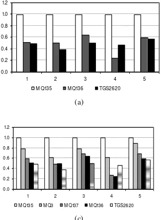
Training data sets used in this study were aroma patterns of tobacco. There were five samples of tobacco, captured by combination of 7-gas sensors, namely MQ135, MQ136, MQ137, MQ138, MQ3, TGS2620, and TGS822. Average pattern of these samples are presented on Figure 6. We prepared five training data sets with different combination of these sensors. Data 1 represented 5 patterns of tobacco captured by combination of 3 sensors. Data 2 was pattern of the sample odor with 4 sensors, data 3 with 5 sensors, data 4 with 6 sensors, and the last data was captured by combination of seven sensors.

III.RESULTS AND DISCUSSION

Both CBPNNs were trained to recognize all data sets. Training was conducted for both neural networks for five repetitions for each data set. Both of them were trained with learning rate of 0.7, momentum of 0.2, and maximum error threshold of 0.001. This study conducted on laptop with specification of Intel Celeron M processor 440 (1.86 GHz, 533 MHz FSB, 1 MB L2 cache) with memory of 1.5 MB DDR2.

Effectiveness of both algorithms (fixed and FL) have been evaluated. There are three components used for this evaluation, i.e. size of final network, number of training iteration, and time of network learning. The network size in general MLP network involves the number of layers and the number of hidden-units per layer. Both of them reflect the complexity of the network. Number of units in each layer presents the numbers of connections in the network. Number of layers indicates the stage of computing process when it trained and used. Normally, the number of units in the input and output layers can be determined by the dimensionality of the problem or training data set, so the number cannot be set up when the network trained. Studying neural network which have determined configuration layer, observation of the network size is focused on the number of neurons in the hidden layer. In this study, the network size is represented by the number of neurons in the hidden layer. Time for training and number of iterations are used to represent the load of learning process. Result of this study is detailed as follows:

A. Training of OHL-CBPNN

OHL-CBPNN was prepared and trained for all data sets. Observation involves size of final network, training iteration, and training time. The result of this study is presented on Table 2. This result written on the table is average value of five experimental data.

From the Table 2, we clearly know that the smaller size of final network is generated by fixed 1 and FL methods. Based on size consideration, result showed that adding more unit numbers simultaneously tends to generate bigger size of the final network. Comparison of both algorithms is clearly understood on Figure 7.

smaller structure is generated by applying smaller new unit number. The study shows that fixed 1 method can construct final network with smaller size. Compare to fixed 1 method, FL method also generate small network. From this result, both methods can be recommended to train the OHL-CBPNN.

Beside size of network, effectiveness of the proposed method is evaluated from number of training iteration. Comparison of iteration number for both methods can be shown on Figure 8. Figure 8 presents that application of both methods does not significantly affect to the number of iteration. The biggest influence is only seen on the OHL-CBPNN with fixed 1 method. Result shows that this method tends to increase number of training iteration. This is understandable because this method cause the structure changed slowly. Based on these results, the FL and fixed method with smaller number of iteration may be selected.

Time of network training is also used to evaluate performance of the proposed algorithm. Training time of the OHL-CBPNN with various data sets is presented on Figure 9. With this result, we know that number of new unit added in the fixed method determines speed of the network convergence. Fixed method with small number of units tends to accelerate its training process. FL method also shows good performance. This method is able to minimize load of computation and results network with high speed of convergence. Compare to the studied method, FL method can be recommended.

Based on the previous parameters, we can conclude that FL methods applied on OHL-CBPNN training shows the best performance. This method can be used to optimize training of the network. This is due to results of training time, training iteration, and network size of the network.

B. Training of DHL-CBPNN

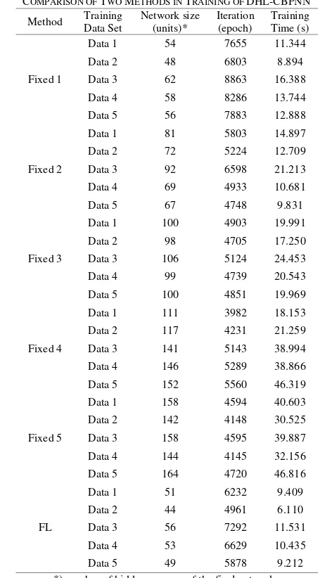
DHL-CBPNN is trained to recognize the same data sets. The similar manner is applied in this experiment in accordance with the previous experimental design. In this study, we also focus to evaluate 3 parameters, i.e. size of network, training time, and iteration. Study result shows on Table 3.

Based on Table 3, we can analyze that both, proposed method and comparison method, show similar performance with the previous study. Smaller size of network is also generated by applying of FL and Fixed 1 methods. Both FL and fixed 1 method may be chosen to generate small CBPNN. Evaluation of network size for both applied algorithm for all variations of data sets is presented on Figure 10. From this result, we consider that both algorithms show the similar characteristic.

Observations of training iteration of DHL-CBPNN are presented in Figure 11. The graph shows that variations of the fixed method employed are not exhibited significantly affects to the network training iterations. The biggest influence can be understood on the implementation of the fixed 1 method. Applying of this method for DHL-CBPNN tends to increase number of training iteration. The result shows that the network convergent with higher number of training iterations than the other methods implemented. This is understandable because the structure development was too slow and each change of structure requires considerable training

iteration. Based on the results, FL method and big new unit number on fixed method can be recommended.

Training time of DHL-CBPNN for both algorithms can be clearly evaluated from Figure 12. The figure shows that training time of the network for all data patterns was determined by implementation of training methods. From the figure, we can conclude that FL method give the best performance due to minimum time of convergence.

Based on the three parameters studied before, we consider that FL method can be used as new strategy on training of DHL-CBPNN. Due to the same result on training of OHL-CBPNN, we sure that this method can be implemented on training of general CBPNN.

C. Analyze of Both Algorithms on Training of OHL-CBPNN and DHL-OHL-CBPNN

In this section, we focus on analyzing performance of FL method compared to fixed methods. In order to evaluate effectiveness of FL method, we only compare the method to the best and average performance of fixed method. Best performance in this section is defined as method, which is able to generate small size of final network with minimum iteration and time. Percentages of network size, training iteration, and training time are discussed. Network size comparison of FL method and related fixed method is presented on Table 4.

Colum A in the Table 4 is smaller network size for all fixed methods implemented in training of CBPNN. Fixed 1 method showed the best performance due to its ability to generate smallest network for all data patterns. We can evaluate the performances of both algorithms by comparing the data. Result shows that FL method implemented on OHL-CBPNN was able to generate smaller network compare to fixed 1 method (94.98 %). Better performance of FL method is showed if we compare it with the average size of final network of various fixed methods. FL method is able to produce less than a half size of final network with fixed method. Similar performance of FL method is also presented on training of DHL-CBPNN. FL method is effective to minimize final network size with average of 91.47 % compared to the best fixed method and 48.71 % compared to average fixed method implemented. This result showed that the proposed method is effective to find minimum network architecture.

Beside network size, performance evaluation of both methods can be evaluated from training iteration. Comparison of training iteration between FL method and related fixed method is presented on Table 5. It shown that fixed method (the best and average) has better performance than FL method for OHL-CBPNN and DHL-CBPNN. CBPNN trained by fixed method is able to convergence with less training iteration than FL method implemented. It can be understood from the design of FL discussed in the previous section.

only 43.96 % of training time used by average fixed method and 14.78 % less than the best fixed method.

The similar result is showed on training of DHL-CBPNN. In this case, the proposed method also presents better performance. The study result shows that the network trained using FL method was able to recognize the data pattern more than two times faster than the average performance of fixed methods studied. The data shows that DHL-CBPNN with FL method is able to convergence with only 39.66 % of average time needed when the fixed method applied and 73.88 % of time needed by the best fixed method implemented.

Based on the study result, we can conclude that FL method is suitable to train not only OHL-CBPNN but also DHL-CBPNN. Although this method tends to add a few number of training iteration, FL method is able to minimize the final network size and time of training.

D. Computational Load of Training

Computational load is mainly used to evaluate effectiveness of an algorithm or method. Computational load is closely related to the algorithm design. A program, which contains a lot of multiplier, is usually difficult to be executed. In this case, the algorithm has high computational load. We also can predict the computational load by evaluating difficulty level of the algorithm. Besides, computational load can also be valued from the computer load when the algorithm is running. Light algorithm is easy to be computed. In this section, we only focus on the effect showed on computer when the both methods implemented on the OHL-CBPNN and DHL-OHL-CBPNN.

In the previous section, we captured training iteration and training time data. Both are used to calculate iteration frequency (f) of training of the neural network. Frequency of iteration means number of iteration for each second, which can be formulated as follows:

t I

f  (21)

where I is number of training iteration and t is total time needed to train the network. Number of f shows the load of computing process.

Comparison of f for both methods implemented on both CBPNN is presented on Table 7. It shown that proposed method has better performance than proper fixed method. Value of iteration frequency of CBPNN trained by FL method is bigger than the similar neural network when fixed method is implemented. It means that FL method tends to reduce load of computational process significantly. Implementation of FL shows that load of processor is lighter than the other methods implemented on training of CBPNN.

These results prove that the addition of the algorithm does not necessarily aggravate the computational load, but in this case, the addition of FL algorithm can decrease load the network training. Thus, we agree that combining FL algorithm on CBPNN does not increase training load, but otherwise, it tends to drop off training load.

IV.CONCLUSION

This paper presented training of CBPNN by implementing FL method and fixed method. The neural network was used to recognize aroma pattern on an electronic nose system. The result shows that FL method applied on OHL-CBPNN and DHL-CBPNN is able to generate small final neural network. Besides that, FL method on both CBPNNs can minimize training time. FL method is also possible to reduce load of computational training. Combining FL method and CBPNN is possible to increase performance of the network. Therefore, this method can be recommended to arrange structure development of general CBPNN.

Input layer

Hidden layer

Output layer

w1 w2

.

.

.

1 1

Output bias Hidden

bias

b1 b2 Input

pattern

x1

x1 . . .

xnInput

Target

t1

t1 . . .

tnOutput

Set of Training Data Network Training

Parameter Start

Accepted Error Design of Initial Network

Design of New Network

Save Final Network

Stop Yes

No

Input layer

Hidden 1 layer

Hidden 2 layer

Output layer Output w1

w2 w3

Bias hidden

Bias hidden

Bias output

. ..

1 1

. ..

1 Input

Network Training Forward

Step

Backward Step

Updating Weight

FL Method MSE

dMSE Fuzzification Inference Defuzzification

Figure 2. FL method implemented on CBPNN

VS S M B VB

10xErrLim 100xErrLim 1000xErrLim nOutput JumData 1

alfa

Figure 3. Memberships function of MSE

S M B

-nOutput -1000xErrLim -10xErrLim 1

alfa

Figure 4. Memberships function of dMSE

VS S M B VB

0 0.1 0.3 0.5 0.7 0.9 1

(a) (b)

(c) (d)

(e)

Figure 6. Patterns of training data set (a) data 1, (b) data 2, (c) data 3, (d) data 4, (e) data 5

Figure 7. Final network size of OHL-CBPNN with fixed and FL methods for all training data sets

Figure 8. Training iteration of OHL-CBPNN with fixed and FL methods for all training data sets

Figure 9. Training time of OHL-CBPNN with fixed and FL methods for all training data sets

Figure 10. Final network size of DHL-CBPNN with fixed and FL methods for all training data sets

0.0 0.2 0.4 0.6 0.8 1.0 1.2

1 2 3 4 5

M Q135 M Q136 TGS2620

0.0 0.2 0.4 0.6 0.8 1.0 1.2

1 2 3 4 5

M Q135 M Q137 M Q136 TGS2620

0.0 0.2 0.4 0.6 0.8 1.0 1.2

1 2 3 4 5

Figure 11. Training Iteration of DHL-CBPNN with fixed and FL methods for all training data sets

Figure 12. Training time of OHL-CBPNN with fixed and FL methods for all training data sets

TABLE 1. RULE OF FL

MSE dMSE

S M B

VS VS S S

S S M M

M M M B

B M B B

VB B VB VB

TABLE 2.

COMPARISON OF TWO METHODS IN TRAINING OF OHL-CBPNN

Method Training _{Data Set} Network size _(units)* Iteration _(epoch) Training _{Time (s)}

Fixed 1

Data 1 105 31095 37.181

Data 2 72 21221 18.834

Data 3 70 20565 17.938

Data 4 82 24221 26.310

Data 5 81 23823 26.119

Fixed 2

Data 1 159 23616 42.719

Data 2 153 22643 41.588

Data 3 117 17321 24.987

Data 4 117 17347 26.335

Data 5 131 19406 33.262

Fixed 3

Data 1 236 23351 61.706

Data 2 213 21127 52.779

Data 3 190 18750 43.878

Data 4 177 17557 39.203

Data 5 191 18885 47.422

Fixed 4

Data 1 295 21959 70.950

Data 2 258 19190 58.865

Data 3 246 18223 54.500

Data 4 240 17885 54.515

Data 5 228 16926 51.113

Fixed 5

Data 1 386 22968 100.162

Data 2 311 18499 67.619

Data 3 298 17675 65.053

Data 4 283 16764 59.931

Data 5 249 14836 48.240

FL

Data 1 96 23565 24.434

Data 2 74 20304 18.944

Data 3 77 21000 21.303

Data 4 67 18099 16.660

Data 5 72 19710 20.303

*) number of hidden neurons of the final networks

TABLE 3.

COMPARISON OF TWO METHODS IN TRAINING OF DHL-CBPNN

Method Training _{Data Set} Network size _(units)* Iteration _(epoch) Training _{Time (s)}

Fixed 1

Data 1 54 7655 11.344

Data 2 48 6803 8.894

Data 3 62 8863 16.388

Data 4 58 8286 13.744

Data 5 56 7883 12.888

Fixed 2

Data 1 81 5803 14.897

Data 2 72 5224 12.709

Data 3 92 6598 21.213

Data 4 69 4933 10.681

Data 5 67 4748 9.831

Fixed 3

Data 1 100 4903 19.991

Data 2 98 4705 17.250

Data 3 106 5124 24.453

Data 4 99 4739 20.543

Data 5 100 4851 19.969

Fixed 4

Data 1 111 3982 18.153

Data 2 117 4231 21.259

Data 3 141 5143 38.994

Data 4 146 5289 38.866

Data 5 152 5560 46.319

Fixed 5

Data 1 158 4594 40.603

Data 2 142 4148 30.525

Data 3 158 4595 39.887

Data 4 144 4145 32.156

Data 5 164 4720 46.816

FL

Data 1 51 6232 9.409

Data 2 44 4961 6.110

Data 3 56 7292 11.531

Data 4 53 6629 10.435

Data 5 49 5878 9.212

*) number of hidden neurons of the final networks

Training Iteration

0 2,000 4,000 6,000 8,000 10,000

Fixed 5 Fixed 4 Fixed 3 Fixed 2 Fixed 1 FL

E

p

o

ch

Data 1 Data 2 Data 3 Data 4 Data 5

Training Time

0 15 30 45 60

Fixed 5 Fixed 4 Fixed 3 Fixed 2 Fixed 1 FL

T

im

e

(s

)

TABLE 4.

FINAL NETWORK SIZE COMPARISON OF FL AND RELATED FIXED METHOD

Network Training

Data set A (unit)

B (unit)

FL (unit)

FL/A (%)

FL/B (%)

OHL-CBPNN

Data 1 105 236 96 91.05 40.45

Data 2 72 201 74 103.06 36.85

Data 3 70 184 77 110.00 41.81

Data 4 82 180 67 81.71 37.22

Data 5 81 176 72 89.11 40.92

Average 82 196 77 94.98 39.45

DHL-CBPNN

Data 1 54 101 51 95.15 50.60

Data 2 48 96 44 92.08 46.27

Data 3 62 112 56 90.26 49.75

Data 4 58 103 53 91.38 51.32

Data 5 56 108 49 88.49 45.62

Average 55 104 51 91.47 48.71

A: Final network size of the best fixed method performance B: Average of final network size of fixed methods used

TABLE 5.

TRAINING ITERATION COMPARISON OF FL AND RELATED FIXED METHOD

Network Training

Data Set

A (epoch)

B (epoch)

FL (epoch)

FL/A (%)

FL/B (%)

OHL-CBPNN

Data 1 22,968 24,598 23,565 102.60 95.80

Data 2 18,499 20,536 20,304 109.76 98.87

Data 3 17,675 18,507 21,000 118.81 113.47

Data 4 16,764 18,755 18,099 107.96 96.50

Data 5 14,836 18,775 19,710 132.85 104.98

Average 18,148 20,234 20,535 114.40 101.92

DHL-CBPNN

Data 1 4,594 5,387 6,232 135.66 115.68

Data 2 4,148 5,022 4,961 119.62 98.78

Data 3 4,595 6,064 7,292 158.69 120.24

Data 4 4,145 5,478 6,629 159.92 121.00

Data 5 4,720 5,553 5,878 124.52 105.86

Average 4,440 5,501 6,198 139.68 112.31

A: Training iteration of the best fixed method performance B: Average of training iteration of fixed methods used

TABLE 6.

TRAINING TIME COMPARISON OF FL AND RELATED FIXED METHOD

Network Training

Data Set A (s)

B (s)

FL (s)

FL/A (%)

FL/B (%)

OHL-CBPNN

Data 1 37.18 62.54 24.43 65.72 39.07

Data 2 18.83 47.94 18.94 100.58 39.52

Data 3 17.94 41.27 21.30 118.76 51.62

Data 4 26.31 41.26 16.66 63.32 40.38

Data 5 26.12 41.23 20.30 77.73 49.24

Average 25.28 46.85 20.33 85.22 43.96

OHL-CBPNN

Data 1 11.34 21.00 9.41 82.95 44.81

Data 2 8.89 18.13 6.11 68.70 33.70

Data 3 16.39 28.19 11.53 70.37 40.91

Data 4 13.74 23.20 10.43 75.92 44.98

Data 5 12.89 27.16 9.21 71.48 33.91

Average 12.65 23.53 9.34 73.88 39.66

TABLE 7.

FREQUENCY ITERATION COMPARISON OF FL AND RELATED FIXED METHOD

Network Training

Data Set A (Hz)

B (Hz)

FL (Hz)

FL/A (%)

FL/B (%)

OHL-CBPNN

Data 1 617.74 393.29 964.43 156.12 245.22

Data 2 982.17 428.39 1071.79 109.12 250.19

Data 3 985.35 448.42 985.76 100.04 219.83

Data 4 637.18 454.57 1086.40 170.50 239.00

Data 5 568.00 455.36 970.76 170.91 213.19

Average 758.09 436.01 1015.83 141.34 233.48

OHL-CBPNN

Data 1 404.96 256.57 662.30 163.55 258.14

Data 2 466.35 277.05 812.03 174.13 293.10

Data 3 280.38 215.15 632.33 225.53 293.90

Data 4 301.59 236.15 635.27 210.64 269.01

Data 5 366.27 204.40 638.07 174.20 312.16

Average 363.91 237.87 676.00 189.61 285.26

A: Iteration frequency of the best fixed method performance B: Average of f of fixed methods used

REFERENCES

[1] T. C. Pearce, S. S. Schiffmen, H. T. Nagle, and J. W. Gardner,

Handbook of Machine Olfaction. New York: WILEY-VCH Verlag GmbH & Co. KgaA., 2003.

[2] H. Yu, J. Wang, C. Yao, H. Zhang, and Y. Yu, “Quality grad identification of green tea using E-nos by CA and ANN”, LWT,

vol. 41, pp. 1268–1273, 2008.

[3] S. Panigrahi, S. Balasubramanian, H. Gu, C. Lague, and M.

March llo, “N ural-network-integrated electronic nose system for

id ntification of spoil d b f”, LWT, vol. 39, pp. 135–145, 2005,. [4] M. H. Purnomo and A. Kurniawan, Supervised Neural Networks

dan Aplikasinya. Yogyakarta: Graha Ilmu, 2006.

[5] Z. B. Shi, T. Yu, Q. Zhao, Y. Li, and Y. B. Lan, “Comparison of

Algorithms for an El ctronic Nos in Id ntifying Liquors”,

Journal of Bionic Engineering, vol. 5, pp. 253–257, 2008. [6] M. L htokangas, “Mod ling ith constructiv backpropagation”,

Neural Networks,vol. 21, pp.707–716, 1999.

[7] M. L htokangas, “Modifi d constructiv backpropagation for

r gr ssion”, Neurocomputing, vol. 35, pp. 113-122, 2000. [8] . S tiono, “Finding minimal n ural networks for business

int llig nc application”. presented at IFSA-AFSS International Conference, Surabaya-Bali Indonesia, 2011.

[9] T. S. Widodo, Sistem Neurofuzzy. Yogyakarta: Graha Ilmu, 2005. [10] Radi, M. Rivai,M. H. Purnomo, “Multi-thread constructive back

propagation n ural n t ork for aroma patt rn classification”, in