Approaching Dual Quaternions
From Matrix Algebra
Federico Thomas
, Member, IEEE
Abstract—Dual quaternions give a neat and succinct way to en-capsulate both translations and rotations into a unified represen-tation that can easily be concatenated and interpolated. Unfortu-nately, the combination of quaternions and dual numbers seems quite abstract and somewhat arbitrary when approached for the first time. Actually, the use of quaternions or dual numbers sepa-rately is already seen as a break in mainstream robot kinematics, which is based on homogeneous transformations. This paper shows how dual quaternions arise in a natural way when approximating 3-D homogeneous transformations by 4-D rotation matrices. This results in a seamless presentation of rigid-body transformations based on matrices and dual quaternions, which permits building intuition about the use of quaternions and their generalizations.
Index Terms—Biquaternions, Cayley factorization, double quaternions, dual quaternions, spatial kinematics, quaternions.
I. INTRODUCTION
I
N 1843, Hamilton definedquaternionsas quadruples of the form a+bi+cj+dk, where i2 =j2 =k2 =ijk=−1,when seeking a new kind of number that would extend the idea of complex numbers [1].
Quaternions were developed independently of their needs for any particular application. The main use of quaternions in the 19th century consisted in expressing physical theories in the no-tation of quaternions. In this context, during the end of the 19th century, researchers working on electromagnetic theory debated about the choice of quaternion or vector notation in their for-mulations. This generated a fierce dispute from about 1880 to 1900, reaching its climax in a series of letters in the journal Nature[2]. Then, quaternions disappeared from view, and their value discredited, having been replaced by the simpler algebra of matrices and vectors. Later on, in the mid-20th century, the development of computing machinery made necessary a reex-amination of quaternions from the standpoint of their utility in computer simulations. The need for efficient simulations of air-craft and missile motions was responsible to a large extent for sparking the renewed interest in quaternions [3]. It was rapidly realized that quaternion algebra yields more efficient algo-rithms than matrix algebra for applications involving rigid-body
Manuscript received March 6, 2013; revised July 5, 2013; accepted November 26, 2013. Date of publication August 22, 2014; date of current version September 30, 2014. This paper was recommended for publication by Associate Editor M. C. Cavusoglu upon evaluation of the reviewers’ comments. This work was supported by the Spanish Ministry of Economy and Competitiveness through the Explora program under Contract DPI2011-13208-E.
The author is with the Institut de Rob`otica i Inform`atica Industrial, 08028 Barcelona, Spain (e-mail: [email protected]).
Digital Object Identifier 10.1109/TRO.2014.2341312
transformations. Nowadays, quaternions play a fundamental role in the representation of spatial rotations and a chapter de-voted to them can be found in nearly every advanced textbook onComputer Vision, Robot Kinematics and Dynamics, or Com-puter Graphics.
Surprisingly, despite their long life, the use of quaternions in engineering is not free from confusions that mainly concern the following.
1) The order of quaternion multiplication:Quaternions are sometimes multiplied in the opposite order than rotation matrices, as in [4]. The origin of this can be found in the way vector coordinates are represented. For example, in [5], a celebrated book onComputer Graphics, point coor-dinates are represented by row vectors instead of column vectors, as is the common practice in Robotics. Then, transformation matrices postmultiply a point vector to produce a new point vector. The result can be confus-ing for anyone approachconfus-ing quaternions for the first time. For more details on this matter, see [6].
2) The way quaternions operate on vectors: Quaternions have been used to rotate vectors in 3-D by essentially sand-wiching a vector in 3-D between a unit quaternion and its conjugate [7, Ch. 17], [8]. Nevertheless, strictly speaking, quaternions cannot operate on vectors. The word vector was introduced by Hamilton to denote the imaginary part of the quaternion, which is different from today’s meaning [9].
3) The nature of the quaternion imaginary units [6], [8]: Hamilton himself contributed to this confusion as he al-ways identified the quaternion units with quadrantal rota-tions, as he called the rotations byπ/2[10, p. 64, art. 71]. Nevertheless, they represent rotations byπ[9].
All these confusions are seriously affecting the progress of quaternions in engineering because, as a result, they are used in recipes for manipulating sequences of rotations without a pre-cise understanding of their meaning. The situation just worsens when working with dual quaternions, an extension of ordinary quaternions that permits encapsulating rotations and translations in a unified representation. Thus, it is not strange that many prac-titioners are still averse to using them despite their undeniable value.
This paper shows how quaternions do naturally emerge from 4-D rotation matrices and how dual quaternions are then derived when approximating 3-D homogeneous transformations by 4-D rotations. As a consequence, all common misunderstand-ings concerning quaternions are cleared up because the derived expressions may be interpreted both as matrix expressions and as quaternions.
A. Quaternions and Rotations inR3andR4
Soon after Hamilton introduced quaternions, he tried to use them to represent rotations inR3 in the same way as complex numbers can be used to represent rotations inR2. Nevertheless, it seems that he was not aware of Rodrigues’ work and his use of quaternions as a description of rotations was wrong. He believed that the expression for a rotated vector was linear in the quaternion rather than quadratic. This passage of the history of quaternions is actually a matter of controversy (see [9], [11], and [12] for details). It is Cayley whom we must thank for the correct development of quaternions as a representation of rotations and for establishing the connection with the results published by Rodrigues three years before the discovery of quaternions [13]. Cayley is also credited to be the first to discover that quaternions could also be used to represent rotations inR4 [14]. Cayley’s results can be used to prove that any rotation inR4is a product of rotations in a pair of orthogonal 2-D subspaces [15]. This factorization, known as Cayley’s factoring of 4-D rotations, was also proved using matrix algebra by Van Elfrinkhof in 1897 in a paper [16] rescued from oblivion by Mebius in [17]. Cayley’s factorization plays a central role in what follows as it provides a bridge between homogeneous transformations and quaternions that remained unnoticed in the past.
B. Quaternions and Their Generalizations
In 1882, Clifford introduced the idea of a biquaternion in three papers: “Preliminary sketch of biquaternions,” “Notes on biquaternions,” and “Further note on biquaternions” [18] (see [19] for a review and summary of these papers). Clifford adopted the word biquaternion, previously used by Hamilton to refer to a quaternion with complex coefficients, to denote a combination of two quaternions algebraically combined via a new symbolω defined to have the propertyω2= 0so that a biquaternion has
the formq1+ωq2, whereq1 andq2 are both ordinary
quater-nions. The use of the term biquaternion is confusing. As ob-served in [19], even Clifford contributed to this confusion by using the symbolωin several different contexts. For example, in his paper “Preliminary sketch of biquaternions,” it is also used with the multiplication ruleω2 = 1. Nowadays, in the area
of robot kinematics, biquaternions of the formq1+εq2, where
ε2 = 0, are called dual quaternions, while those of the form
q1+eq2, where e2 = 1, are called double quaternions. This
denomination derives from the fact that the symbols ε ande designate thedualand thedoubleunits, respectively [20]. Thus, we have three imaginary units, which can be equal either to the complex uniti(i2 =−1), to the dual unitε(ε2= 0), or to
the double unite(e2 = 1). These units define the basis of the
so-called hypercomplex numbers [21].
The double quaternion q1+eq2 can be reformulated by
introducing the symbols ξ= 1+e2 and η=1−2e [18], [22]. Then,q1+eq2 =ξ(q1+q2) +η(q1−q2). Sinceξ2 =ξ,η2 =
η, andξη= 0, the terms(q1+q2)and(q1−q2)operate
inde-pendently in the double quaternion product, which has been found quite convenient when manipulating kinematic equations expressed in terms of double quaternions [23]. A third pos-sible representation for double quaternions consists in having
two quaternions expressed in different bases of imaginary units whose product is commutative. This also leads to couples of quaternions that operate independently when multiplied. Nowa-days, the algebras of ordinary, double, and dual quaternions are grouped under the umbrella of Clifford algebras, also known as geometric algebras (see [24, Ch. 9] or [25] for an introduction). While double quaternions have found direct application to represent 4-D rotations, dual quaternions found application to encapsulate both translation and rotation into a unified represen-tation. Then, if 3-D spatial displacements are approximated by 4-D rotations, a beautiful connection between double and dual quaternions can be established.
Yang and Freudenstein introduced the use of dual quaternions for the analysis of spatial mechanisms [26]. Since then, dual quaternions have been used by several authors in the kinematic analysis and synthesis of mechanisms, and in computer graphics (see, for instance, the works of McCarthy [27], Angeles [28], and Perez-Gracia [29]).
C. Quaternions and Matrix Algebra
Matrix algebra was developed in the beginning of 1858 by Cayley and Sylvester. Soon it was realized that matrices could be used to represent the imaginary units used in the definition of quaternions. Actually, a set of4×4matrices, sometimes called Dirac–Eddington–Conway matrices, with real values can realize every algebraic requirement of quaternions. Alternatively, a set of2×2matrices, usually called Pauli matrices, with complex values can play the same role (see [30, pp. 143–144] for details). Therefore, there are sets of matrices, which all produce valid matrix representations of quaternions. The choice of one set over other has been driven by esthetic preferences, but we will show how Cayley’s factorization leads to a matrix representation that attenuates this sense of arbitrariness.
While in most textbooks, the matrix representation of quater-nions is considered as an advanced topic, if ever mentioned, in this paper, matrix algebra is used as the doorway to quaternions. This would probably be the usual practice if matrix algebra had been developed before quaternions.
D. Organization of the Paper
examples, and, finally, we conclude in Section VIII with a sum-mary of the main points.
II. FOUR-DIMENSIONALROTATIONS ANDDOUBLEQUATERNIONS
After a proper change in the orientation of the reference frame, an arbitrary 4-D rotation matrix (i.e., an orthogonal matrix with determinant+1) can be expressed as [31, Th. 4]:
⎛ ⎜ ⎜ ⎝
cosα1 −sinα1 0 0
sinα1 cosα1 0 0
0 0 cosα2 −sinα2
0 0 sinα2 cosα2
⎞ ⎟ ⎟
⎠. (1)
Thus, a 4-D rotation is defined by two mutually orthogonal planes of rotation, each of which is fixed in the sense that points in each plane stay within the planes. Then, a 4-D rotation has two angles of rotation,α1andα2, one for each plane of rotation,
through which points in the planes rotate. All points not in the planes rotate through an angle betweenα1 and α2. See [32]
for details on the geometric interpretation of rotations in four dimensions.
Ifα1 =±α2, the rotation is called anisoclinic rotation. An
isoclinic rotation can beleft- orright-isoclinic(depending on whether α1 =α2 or α1 =−α2, respectively), which can be
represented by a rotation matrix of the form
RL =
⎛ ⎜ ⎜ ⎝
l0 −l3 l2 −l1
l3 l0 −l1 −l2 −l2 l1 l0 −l3
l1 l2 l3 l0
⎞ ⎟ ⎟
⎠ (2)
and
RR =
⎛ ⎜ ⎜ ⎝
r0 −r3 r2 r1
r3 r0 −r1 r2 −r2 r1 r0 r3 −r1 −r2 −r3 r0
⎞ ⎟ ⎟
⎠ (3)
respectively. Since (2) and (3) are rotation matrices, their rows and columns are unit vectors. As a consequence
l2
0+l12+l22+l23 = 1 (4)
and
r20+r02+r02+r32 = 1. (5)
Without loss of generality, we have introduced some changes in the signs and indices of (2) and (3) with respect to the notation used by Cayley [14], [33] to ease the treatment given below and to provide a neat connection with the standard use of quaternions for representing rotations in three dimensions.
Isoclinic rotation matrices have three important properties. 1) The product of two right- (left-) isoclinic matrices is a
right- (left-) isoclinic matrix.
2) The product of a right- and a left-isoclinic matrix is com-mutative.
3) Any 4-D rotation matrix, according to Cayley’s factoriza-tion, can be decomposed into the product of a right- and a left-isoclinic matrix.
Then, a 4-D rotation matrix, sayR, can be expressed as
R=RLRR =RRRL (6)
where
RL =l0I+l1A1+l2A2+l3A3 (7)
and
RR =r0I+r1B1+r2B2+r3B3 (8)
whereIstands for the4×4identity matrix and
A1 =
⎛ ⎜ ⎜ ⎝
0 0 0 −1 0 0 −1 0 0 1 0 0 1 0 0 0
⎞ ⎟ ⎟
⎠, A2 =
⎛ ⎜ ⎜ ⎝
0 0 1 0 0 0 0 −1
−1 0 0 0
0 1 0 0
⎞ ⎟ ⎟ ⎠
A3 =
⎛ ⎜ ⎜ ⎝
0 −1 0 0 1 0 0 0 0 0 0 −1 0 0 1 0
⎞ ⎟ ⎟
⎠, B1 =
⎛ ⎜ ⎜ ⎝
0 0 0 1 0 0 −1 0 0 1 0 0
−1 0 0 0
⎞ ⎟ ⎟ ⎠
B2 =
⎛ ⎜ ⎜ ⎝
0 0 1 0 0 0 0 1
−1 0 0 0
0 −1 0 0
⎞ ⎟ ⎟
⎠, B3 =
⎛ ⎜ ⎜ ⎝
0 −1 0 0 1 0 0 0 0 0 0 1 0 0 −1 0
⎞ ⎟ ⎟
⎠.
Therefore,{I,A1,A2,A3}and{I,B1,B2,B3}can be seen,
respectively, as bases for left- and right-isoclinic rotations. The details on how to compute Cayley’s factorization (6) can be found in the Appendix.
Now, it can be verified that
A21 =A22 =A23 =A1A2A3 =−I (9)
and
B21 =B22 =B23 =B1B2B3=−I. (10)
We can recognize in these two expressions the quaternion def-inition. Actually, (9) and (10) reproduce the celebrated formula that Hamilton carved into the stone of Brougham bridge.
Expression (9) determines all the possible products of A1, A2, andA3resulting in
A1A2 = A3, A2A3 =A1, A3A1 =A2
A2A1 = −A3, A3A2 =−A1, A1A3 =−A2. (11) Likewise, all the possible products ofB1,B2, andB3can be
derived from expression (10). All these products can be sum-marized in the following product tables:
I A1 A2 A3
I I A1 A2 A3
A1 A1 −I A3 −A2
A2 A2 −A3 −I A1
A3 A3 A2 −A1 −I
I B1 B2 B3
I I B1 B2 B3
B1 B1 −I B3 −B2
B2 B2 −B3 −I B1
B3 B3 B2 −B1 −I
(13)
Moreover, it can be verified that
AiBj =BjAi (14)
which is actually a consequence of the commutativity of left-and right-isoclinic rotations. Then, in the composition of two 4-D rotations, we have
R1R2= (RL1RR1)(RL2R2R) = (RL1RL2)(RR1RR2). (15)
It can be concluded thatRLi andRRi can be seen either as 4×4 rotation matrices or, when expressed as in (7) and (8), respectively, as unit quaternions and their product, as a double quaternion because they operate independently in the product of two 4-D rotations. It is said that they are unit quaternions because their coefficients satisfy (4) and (5).
Next, in Section IV, the above twofold matrix-quaternion rep-resentation of 4-D rotations is specialized to 3-D rotations and, in Section V, generalized to represent 3-D translations. Nev-ertheless, let us fist explore this twofold representation a bit further.
III. DIGRESSION
One of the multiple advantages of the proposed matrix-quaternion formulation is that the involved imaginary units have a clear algebraic interpretation. We can operate with these units to obtain different representations of 4-D rotations that would otherwise be quite abstract and difficult to derive. To see this, let us start by defining
D1 =A1B−11 =
⎛ ⎜ ⎜ ⎝
−1 0 0 0
0 1 0 0 0 0 1 0 0 0 0 −1
⎞ ⎟ ⎟ ⎠
D2 =−A2B−21 =
⎛ ⎜ ⎜ ⎝
1 0 0 0 0 −1 0 0 0 0 1 0 0 0 0 −1
⎞ ⎟ ⎟ ⎠
D3 =A3B−31 =
⎛ ⎜ ⎜ ⎝
−1 0 0 0
0 −1 0 0 0 0 1 0 0 0 0 1
⎞ ⎟ ⎟
⎠.
Then, it can be verified that
D21 =D22 =D32=D1D2D3 =I (16)
which allow us to define a kind of quaternion whose imaginary units are double units. As with ordinary quaternions, (16) deter-mines all the possible products ofD1,D2, andD3, which can
be summarized in the following product table:
I D1 D2 D3
I I D1 D2 D3
D1 D1 I D3 D2
D2 D2 D3 I D1
D3 D3 D2 D1 I.
(17)
Then, clearlyDi=D−i1,i= 1,2,3, and, as a consequence B1 =D1A1, B2 =−D2A2, and B3 =D3A3. Substituting the above expressions forBi, i= 1,2,3, in (8),
multiplying the result by (7), and factoring outDi,i= 1,2,3,
we conclude that (6) can be rewritten as
R=IQ0+D1Q1+D2Q2+D3Q3 (18)
where
Q0 = r0(l0I+l1A1+l2A2+l3A3) Q1 = r1(l0A1−l1I+l2A3−l3A2) Q2 = r2(−l0A2+l1A3+l2I−l3A1) Q3 = r3(l0A3+l1A2−l2A1−l3I).
Now, we can shift from the basis{I,D1,D2,D3}to the basis {E1,E2,E3,E4}defined as
E1 = 1
4(I−D1 +D2−D3) =
⎛ ⎜ ⎜ ⎝
1 0 0 0 0 0 0 0 0 0 0 0 0 0 0 0
⎞ ⎟ ⎟
⎠ (19)
E2 =
1
4(I+D1 −D2−D3) =
⎛ ⎜ ⎜ ⎝
0 0 0 0 0 1 0 0 0 0 0 0 0 0 0 0
⎞ ⎟ ⎟
⎠ (20)
E3 = 1
4(I+D1 +D2+D3) =
⎛ ⎜ ⎜ ⎝
0 0 0 0 0 0 0 0 0 0 1 0 0 0 0 0
⎞ ⎟ ⎟
⎠ (21)
E4 =
1
4(I−D1−D2+D3) =
⎛ ⎜ ⎜ ⎝
0 0 0 0 0 0 0 0 0 0 0 0 0 0 0 1
⎞ ⎟ ⎟
⎠. (22)
The elements of this basis are distinguished by the fact that their multiplication table is the simplest possible for a basis
E1 E2 E3 E4
E1 E1 0 0 0
E2 0 E2 0 0
E3 0 0 E3 0
E4 0 0 0 E4.
By inverting the system of equations defined by (19)–(22), we obtain
D1 = −E1+E2+E3−E4
D2 = E1 −E2+E3−E4
D3 = −E1−E2+E3+E4.
Substituting these expressions into (18) and factoring outEi,
fori= 1, . . . ,4, we obtain
R=E1K1+E2K2+E3K3+E4K4 (23)
where
K1 = Q0−Q1+Q2−Q3
= (r0l0+r1l1+r2l2+r3l3)I
+(r0l1−r1l0−r2l3+r3l2)A1
+(r0l2+r1l3−r2l0−r3l1)A2
+(r0l3−r1l2+r2l1−r3l0)A3 K2 = Q0+Q1−Q2−Q3
= (r0l0−r1l1−r2l2+r3l3)I
+(r0l1+r1l0+r2l3+r3l2)A1
+(r0l2−r1l3+r2l0−r3l1)A2
+(r0l3+r1l2−r2l1−r3l0)A3 K3 = Q0+Q1+Q2+Q3
= (r0l0−r1l1+r2l2−r3l3)I
+(r0l1+r1l0−r2l3−r3l2)A1
+(r0l2−r1l3−r2l0+r3l1)A2
+(r0l3+r1l2+r2l1+r3l0)A3
and
K4 = Q0−Q1−Q2+Q3
= (r0l0+r1l1−r2l2−r3l3)I
+(r0l1−r1l0+r2l3−r3l2)A1
+(r0l2+r1l3+r2l0+r3l1)A2
+(r0l3−r1l2−r2l1+r3l0)A3.
It is thus concluded that a 4-D rotation can be expressed as a linear combination of four quaternions. In the product of two 4-D rotations, these four quaternions operate independently becauseE2i =Ei, fori= 1,2,3,4, andEiEj =0ifi=j. The
reader interested in further exploring the connections between 4-D rotations and different sets of imaginary units is referred to [33] and [34].
IV. THREE-DIMENSIONALROTATIONS ANDORDINARYQUATERNIONS
We have seen how double quaternions naturally emerge from Cayley’s factorization of 4-D rotations into isoclinic rotations. Now, we specialize this result to 3-D rotations.
The homogenous matrix transformation representing a rota-tion byφabout thexaxis is
Rx(φ) =
⎛ ⎜ ⎜ ⎝
1 0 0 0
0 cos(φ) −sin(φ) 0 0 sin(φ) cos(φ) 0
0 0 0 1
⎞ ⎟ ⎟
⎠ (24)
which can be readily interpreted as a rotation inR4. Then, its Cayley’s factorization into a right- and a left-isoclinic rotation, using the procedure given in the Appendix, yields
RLx(φ) =√ 1
t2+ 1
⎛ ⎜ ⎜ ⎝
1 0 0 −t 0 1 −t 0 0 t 1 0 t 0 0 1
⎞ ⎟ ⎟
⎠ (25)
and
RRx(φ) = √ 1
t2+ 1
⎛ ⎜ ⎜ ⎝
1 0 0 t 0 1 −t 0 0 t 1 0
−t 0 0 1
⎞ ⎟ ⎟
⎠ (26)
respectively, where we have introduced the change of variable t= tanφ2 to obtain more amenable expressions. Then
Rx(φ) =
1
√
t2+ 1(I+tA1)
1
√
t2+ 1(I+tB1)
. (27) We can perform the same factorization for rotations about the y- and thez-axes. Table I compiles the results.
Now, let us suppose that we want to represent a general rota-tion using theXYZCardanian angles [35, p. 28]. Then
Rx(φ1)Ry(φ2)Rz(φ3)
=
1
t2 1+ 1
(I+t1A1)
1
t2 1+ 1
(I+t1B1)
1
t2 2+ 1
(I+t2A2) 1
t2 2+ 1
(I+t2B2)
1
t2 3+ 1
(I+t3A3)
1
t2 3+ 1
(I+t3B3)
.
Therefore, using the commutativity of left- and right-isoclinic rotations, and the product tables (12) and (13), we conclude that
Rx(φ1)Ry(φ2)Rz(φ3) =Q1Q2=Q2Q1 (28)
where
Q1 =
1
(t2
1+ 1)(t22+ 1)(t23+ 1)
[(1−t1t2t3)I
+(t1+t2t3)A1+ (t2−t1t3)A2+ (t3+t1t2)A3]
and
Q2 = 1
(t2
1+ 1)(t22+ 1)(t23+ 1)
[(1−t1t2t3)I
TABLE I
THREE-DIMENSIONALROTATIONS INHOMOGENEOUSCOORDINATESINTERPRETED AS4-D ROTATIONS ANDTHEIRFACTORIZATIONSINTO
LEFT-ANDRIGHT-ISOCLINICROTATIONS(t= tan(φ2))
Transformation Left-Isoclinic Right-Isoclinic Double Quaternion
Rx(φ) =
INFINITESIMAL3-D TRANSLATIONS INHOMOGENEOUSCOORDINATESAPPROXIMATED BY4-D ROTATIONS ANDTHEIRFACTORIZATIONSINTO
LEFT-ANDRIGHT-ISOCLINICROTATIONS
Transformation Left-Isoclinic Right-Isoclinic Double Quaternion
Txdδδ
Similar results are obtained for other sets of Eulerian or Car-danian angles. In any case, after constraining rotations to three dimensions, the double quaternion representation becomes re-dundant as one quaternion can be deduced from the other by simply exchanging Ai and Bi. Thus, a 3-D rotation can be
represented either by a quaternion of the form(p0I+p1A1+
p2A2+p3A3)or(p0I+p1B1+p2B2+p3B3)and the
cor-responding homogeneous matrix can be obtained by computing their commutative product. Indeed, it can be verified that
(p0I+p1A1+p2A2+p3A3)(p0I+p1B1+p2B2+p3B3)
Observe that this is the well-known formula that permits pass-ing from a quaternion representation to the correspondpass-ing rota-tion matrix [7, p. 85].
Now, if we substitute into (29) the following values:
p0 = cos
This alternative to Rodrigues’ formula provides a seamless connection between homogeneous transformations and nions that can easily be grasped by anyone approaching quater-nions for the first time. This formula also demonstrates two important concepts. First, a 3-D rotation can be seen as the composition of two 4-D isoclinic rotations. Second, contrary to popular belief, a unit quaternion actually represents a 4-D rota-tion (see [37], for an alternative proof of these two facts using heavier mathematical machinery).
Equation (30) is also interesting because it can be concluded from it that Cayley’s factorization gives the axis-angle repre-sentation of a 3-D rotation.
Notice that we can operate withAiandBi,i= 1, . . . ,3, as
symbols whose products commute and satisfy the product tables (12) and (13). We do not need to substitute for them by their corresponding matrices unless we explicitly need the matrix representation. Keeping them as symbols has benefits in three important practical applications:
1) to generate more compact expressions involving rotations and, in general, to increase speed and reduce storage for calculations involving long sequences of rotations, 2) to avoid distortions arising from numerical inaccuracies
caused by floating point computations with rotations, and 3) to interpolate between two rotations for generating trajec-tories. The interpolation of two quaternions still represents a valid rotation contrarily to what happens when interpo-lating two rotation matrices.
Actually, these are the well-known advantages of using quaternions. For their detailed analysis, see [30, Ch. IX].
V. THREE-DIMENSIONALTRANSLATIONS ANDDUALQUATERNIONS
Let us suppose that we want to obtain the nearest rotation matrix, under the Frobenius norm, to a given homogeneous transformation matrixM. To find this rotation matrix, sayR, we can use the singular value decompositionM=U Σ VT to writeR=UVT [38], [39].
If we compute the singular value decomposition of the ho-mogeneous transformation matrix representing an infinitesimal translation along thex-axis, we obtain
⎛
Then, the nearest (in Frobenious norm) 4-D rotation matrix approximating an infinitesimal translation along the x-axis in
homogeneous coordinates is given by
⎛
which can be factored into the product of a right- and a left-isoclinic rotation. The same can be performed for infinitesimal translations along the other coordinate axes. Table II compiles the results.
Now, let us suppose that we perform an infinitesimal transla-tion in the directransla-tion given by the vectort= (tx, ty, tz)T. Then Using the product tables (12) and (13) and neglecting higher order infinitesimals, we conclude that
Tx
An alternative way to perform the above operation in a more elegant way is by introducing the symbol ε,ε2 = 0 (i.e., the
dual unit). It can actually be shown that
Tx(εtx)Ty(εty)Tz(εtz)
In other words,εdpermits working as ifdwere infinitely small without explicitly having to compute limits. Therefore, based on (31), we can establish the following one-to-one correspondence between general 3-D translations expressed as homogeneous transformation matrices and a subset of 4-D rotation matrices
Observe that we have dropped the 1/2 term as it is just a constant scaling factor.
Since any arbitrary rigid motion can be expressed as a trans-lation followed by a rotation, the above correspondence induces the following correspondence between general 3-D rigid mo-tions expressed as homogeneous transformation matrices and 4-D rotation matrices
I3×3 t
0T 1
R3×3 0
0T 1
I3×3 εt
εtT 1
R3×3 0
0T 1
R3×3 t
0T 1
F ⇄ F−1
R3×3 εt
εtTR3×3 1
. (33)
From now on, we will denote M=F(M), where M is an arbitrary transformation matrix. Observe that F(M1M2) = F(M1)F(M2). From this property, one can deduce thatFmaps
the identity element into the identity element, and it also maps inverses to inverses in the sense thatF(M−1) = (F(M))−1.
Technically speaking,Fis a group isomorphism [40, Sec. 2.2]. At this point, it is important to realize that the 4-D rotation ma-trix corresponding to a 3-D homogeneous transformation mama-trix throughFis not an approximation, it is an exact representation, and that the use of dual numbers to represent general 3-D trans-lations in terms of 4-D rotation matrices is completely different from the standard approach based on 3-D rotation matrices [41]– [43]. The use given here, while allowing a clear-cut distinction between translations and rotations, provides at the same time a neat connection with standard homogeneous transformations.
Now, the 4-D rotation matrix corresponding to the translation in the direction given by the unit vectorn= (nx, ny, nz)T a
distanced, after factoring it using Cayley’s factorization, can be expressed as
Tn(d) =
I−εd
2(nxA1+nyA2+nzA3)
I+εd
2(nxB1+nyB2+nzB3)
. (34) As with 3-D rotations, the double quaternion representation of 3-D translations is also redundant because one quaternion can be deduced from the other by exchangingAi andBi and
changing the sign of the dual part.
VI. KINEMATICEQUATIONS
Consider the kinematic equation:
M0 =M1M2· · ·Mn (35)
whereMi,i= 0, . . . , n, is an arbitrary transformation in
homo-geneous coordinates. This kinematic equation can be translated, through the mapping in (33), into a kinematic equation fully expressed in terms of 4-D rotation matrices. That is
M0 =M1M2· · ·Mn. (36)
Then, using Cayley’s factorization, we obtain
ML0MR0 =ML1MR1 ML2MR2 · · ·MLnMRn. (37)
Therefore, using the properties of left- and right-isoclinic rota-tions, we conclude that
ML0 = ML1 ML2 · · ·MLn (38)
MR0 = MR1 MR2 · · ·MRn. (39) Each rotation matrix in (38), or (39), can readily be inter-preted as a quaternion if expressed in the basis{I,A1,A2,A3},
or{I,B1,B2,B3}. Moreover, as we have already seen, any of
these two equations can be obtained from the other by exchang-ingAiandBiand changing the sign of the dual symbol.
Although translations and rotations provide the basic build-ing blocks of any kinematic equation, in many applications, it is interesting to have a more compact expression for motions combining a rotation about an axis and a translation in the di-rection given by the same axis (i.e., screw motions). Indeed, if we define
S=Rn(θ)Tn(d) (40)
then
SR =
cos
θ 2
−εd
2sin
θ 2
I
+
sin
θ 2
+εd 2cos
θ 2
×(nxB1+nyB2+nzB3).
(41)
Since all powers greater or equal to two of ε vanish, the Taylor expansion off(a+εb)aboutayieldsf(a) +εbf′(a).
As a consequence,sin(a+εb) = sina+εbcosaandcos(a+ εb) = cosa−εbsina[43, p. 3]. Therefore, (41) can be more compactly expressed as
SR = cos
ˆ θ 2
I+ sin
ˆ θ 2
(nxB1+nyB2+nzB3) (42)
whereθˆ=θ+εd. The dual quaternion (42) is undoubtedly a much more compact representation of a screw motion than the expansion of (40). Thus, it is not surprising that dual quater-nions defining successive screw displacements are introduced to simplify the structure of the design equations in the synthesis of mechanisms [29].
The screw displacement given by (42) is not general as the rotation axis passes through the origin. The general form is derived as an example in the next section.
VII. EXAMPLES
The following examples illustrate different aspects on how to operate with the presented twofold matrix-quaternion formalism.
A. Derivation of the Sandwich Formula
unit vector, then
Rq(θ) =C Rp(θ)CT. (43) If we substitute (30) in (43), setθ=π, and separate left- and right-isoclinic rotations, we obtain
(qxA1+qyA2+qzA3)
=CL(pxA1+pyA2+pzA3)(CL)T (44)
and
(qxB1+qyB2+qzB3)
=CR(pxB1+pyB2+pzB3)(CR)T (45)
respectively.
Observe that either (44) or (45), after expressingCRandCL
in quaternion form according to (2) and (3), respectively, is the well-known quaternion sandwich formula used to rotate vectors. It is interesting to observe the number of pages devoted to the derivation of this formula in current textbooks [4, pp. 127–134], [7], and the existence of recent papers essentially devoted to its justification [8], while its derivation using the proposed twofold matrix-quaternion formulation seems much easier, at least for those used to work with homogenous transformations.
B. Approximating Dual Quaternions by Double Quaternions
Let us suppose that we need to obtain the quaternion rep-resentation of the following transformation in homogeneous coordinates:
M= Tx(4)Ty(−3)Tz(7)Ry
π
2 Rz
π
2
=
⎛ ⎜ ⎜ ⎝
0 0 1 4 1 0 0−3 0 1 0 7 0 0 0 1
⎞ ⎟ ⎟
⎠. (46)
The 4-D rotation matrix resulting from the mapping in (33) is
M=
⎛ ⎜ ⎜ ⎝
0 0 1 4ε 1 0 0 −3ε 0 1 0 7ε 3ε −7ε −4ε 1
⎞ ⎟ ⎟
⎠. (47)
Cayley’s factoring of this matrix into left- and right-isoclinic rotation matrices, using the procedure given in the Appendix, yields
ML =
⎛ ⎜ ⎜ ⎝
0.5 + 2ε −0.5 + 3.5ε 0.5 −0.5−1.5ε 0.5−3.5ε 0.5 + 2ε −0.5−1.5ε −0.5
−0.5 0.5 + 1.5ε 0.5 + 2ε −0.5 + 3.5ε 0.5 + 1.5ε 0.5 0.5−3.5ε 0.5 + 2ε
⎞ ⎟ ⎟ ⎠
= (0.5 + 2ε)I+ (0.5 + 1.5ε)A1+ 0.5A2+ (0.5−3.5ε)A3
(48) and
MR =
⎛ ⎜ ⎜ ⎝
0.5−2ε −0.5−3.5ε 0.5 0.5−1.5ε 0.5 + 3.5ε 0.5−2ε −0.5 + 1.5ε 0.5
−0.5 0.5−1.5ε 0.5−2ε 0.5 + 3.5ε
−0.5 + 1.5ε −0.5 −0.5−3.5ε 0.5−2ε
⎞ ⎟ ⎟ ⎠
= (0.5−2ε)I+ (0.5−1.5ε)B1+ 0.5B2+ (0.5 + 3.5ε)B3
(49)
respectively. Hence
M=MLMR = [(0.5 + 2ε)I+ (0.5 + 1.5ε)A1
+ 0.5A2 + (0.5−3.5ε)A3]
[(0.5−2ε)I+ (0.5−1.5ε)B1
+ 0.5B2+ (0.5 + 3.5ε)B3].
This double quaternion representation is redundant as one quaternion can be deduced from the other by exchanging Ai
and Bi and changing the sign of the dual part. Thus, either
the dual quaternion (48) or (49) unambiguously represents the transformation (46).
The rotation matrixMis an exact representation ofM, it is not an approximation. Alternatively, if we are not interested in using dual numbers, we can approximateMby
M =
⎛ ⎜ ⎜ ⎝
0 0 1 4/δ 1 0 0 −3/δ 0 1 0 7/δ 3/δ −7/δ −4/δ 1
⎞ ⎟ ⎟
⎠ (50)
whereδis a scaling factor.M is closer to a 4-D rotation matrix asδtends to infinity (it can be verified that(M) = 1−5/δ2).
This is the approach pioneered in [44] and [45] to approximate 3-D homogeneous transformations by 4-D rotation matrices and used, for example, in [23] in dimensional synthesis, or in [46] to solve the inverse kinematics of a 6R robot. This kind of approximation introduces a tradeoff between numerical stability and accuracy of the approximation (see [45] for details). If we
factorMinto a left- and a right-isoclinic rotation, withδ= 100, we obtain
M L
=
⎛ ⎜ ⎜ ⎝
0.5204 −0.4632 0.4996 −0.5152 0.4632 0.5204 −0.5152 −0.4996
−0.4996 0.5152 0.5204 −0.4632 0.5152 0.4996 0.4632 0.5204
⎞ ⎟ ⎟ ⎠
= 0.5204I+ 0.5152A1+ 0.4996A2+ 0.4632A3
(51)
and
M R
=
⎛ ⎜ ⎜ ⎝
0.4804 −0.5332 0.4996 0.4852 0.5332 0.4804 −0.4852 0.4996
−0.4996 0.4852 0.4804 0.5332
−0.4852 −0.4996 −0.5332 0.4804
⎞ ⎟ ⎟ ⎠
= 0.4804I+ 0.4852B1+ 0.4996B2+ 0.5332B3.
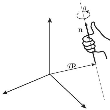
Fig. 1. Geometric parameters used to describe a general screw motion.
Hence, M L
M R
can be used as an approximation ofM
by properly scaling the translations. This approximate double quaternion representation ofMis not redundant as one quater-nion cannot be deduced from the other.
C. Computation of Screw Parameters
Chasles’ theorem states that the general spatial motion of a rigid body can produce a rotation about an axis and a translation along the direction given by the same axis. Such a combination of translation and rotation is called a general screw motion [47]. In the definition of screw motion, a positive rotation corresponds to a positive translation along the screw axis by the right-hand rule.
In Fig. 1, a screw axis is defined byn= (nx, ny, nz)T, a unit
vector defining its direction andqp, the position vector of a point lying on it, wherep= (px, py, pz)T is also a unit vector. The
angle of rotation θand the translational distancedare called the screw parameters. These screw parameters together with the screw axis completely define the general displacement of a rigid body. In terms of homogeneous transformations, in a way similar to (43), this can be expressed as
S=Tp(q)Rn(θ)Tn(d)Tp(−q). (53) Then, using (34) and (42)
∼
SR = I+εq
2(pxB1+pyB2+pzB3)
cos
ˆ θ 2
I+ sin
ˆ θ 2
(nxB1+nyB2+nzB3)
I−εq
2(pxB1+pyB2+pzB3)
(54)
whereθˆ=θ+εd. This can be rewritten, after simplification, as
∼ SR = cos
ˆ θ 2
I+ sin
ˆ θ 2
(ˆnxB1+ ˆnyB2+ ˆnzB3)
(55)
whereˆn= (ˆnx,nˆy,nˆz)T =n+ε qp×n.
Thus, using the presented formalism, the derivation of the screw parameters of an arbitrary 3-D transformation in homoge-nous coordinates entails finding the corresponding 4-D rotation matrix through the mapping (33), obtaining its Cayley’s fac-torization and, finally, identifying the resulting right-isoclinic rotation with (55). For example, to obtain the screw parameters of (46), we have to identify (49) with (55). This identification yields
cos
ˆ θ 2
= 0.5−2ε (56)
ˆ nxsin
ˆ θ 2
= 0.5−1.5ε (57)
ˆ nysin
ˆ θ 2
= 0.5 (58)
ˆ nzsin
ˆ θ 2
= 0.5 + 3.5ε. (59)
From (56), we have that θˆ=θ+εd=23π+ε√8
3. Then,
substituting this value into (57)–(59), we conclude that n= (√1
3, 1 √ 3,
1 √
3)
T andqp×n= (−6√3−1 6 ,−
1 6,
14√3−1 6 )T.
The conversion of a transformation in homogeneous coordi-nates to its corresponding dual quaternion counterpart has tradi-tionally been performed by computing its screw parameters [48, p. 100]. We have shown how Cayley’s factorization performs this task in a more straightforward way. Actually, the screw parameters can be seen as a by-product of this factorization.
VIII. CONCLUSION
We have presented a twofold matrix-quaternion formalism for the representation of rigid-body transformations that permits a better understanding of what dual quaternions are and how they can be manipulated. This formalism stems from Cayley’s factorization of 4-D rotation matrices whose use has been crucial for at least the following three reasons.
1) Cayley’s factorization leads to a matrix representation of quaternions that alleviates the sense of arbitrariness that has dominated the representation of quaternions using ma-trices.
2) Cayley’s factorization, together with a new one-to-one correspondence between 3-D homogeneous transforma-tion matrices and 4-D rotatransforma-tion matrices, permits deriving dual quaternions from homogeneous transformations in a way that a deeper understanding of dual quaternions can be attained.
Thus, Cayley’s factorization certainly deserves a more promi-nent place in the arsenal of the applied kinematician. This paper can ultimately be seen as a vindication of its importance.
APPENDIX
CAYLEY’SFACTORIZATION OF4-D ROTATIONMATRICES
The problem of factoring a 4-D rotation matrix, sayS, into the product of a right- and a left-isoclinic rotation matrices consists in finding the values ofl0, . . . , l3andr0, . . . , r3that satisfy the
following matrix equation:
S=
⎛ ⎜ ⎜ ⎝
s11 s12 s13 s14
s21 s22 s23 s24
s31 s32 s33 s34
s41 s42 s43 s44
⎞ ⎟ ⎟ ⎠
=
⎛ ⎜ ⎜ ⎝
l0 −l3 l2 −l1
l3 l0 −l1 −l2 −l2 l1 l0 −l3
l1 l2 l3 l0
⎞ ⎟ ⎟ ⎠ ⎛ ⎜ ⎜ ⎝
r0 −r3 r2 r1
r3 r0 −r1 r2 −r2 r1 r0 r3 −r1 −r2 −r3 r0
⎞ ⎟ ⎟
⎠.
(60)
According to [33], this problem was first solved by Rosen, a close collaborator of Einstein, in [49].
Equation (60) can be rewritten as
⎛ ⎜ ⎜ ⎝
l0r0 l0r1 l0r2 l0r3
l1r0 l1r1 l1r2 l1r3
l2r0 l2r1 l2r2 l2r3
l3r0 l3r1 l3r2 l3r3
⎞ ⎟ ⎟ ⎠
= 1 4
⎛ ⎜ ⎜ ⎝
s11+s22+s33+s44 s31+s42−s13−s24
s41+s32−s23−s14 −s21−s12−s43−s34 −s31+s42+s13+s24 s11−s22+s33−s44
s21−s12+s43−s34 s41−s32−s23+s14 −s41+s32−s23+s14 s21−s12−s43+s34
s21+s12−s43−s34 s41+s32+s23+s14
s11−s22−s33+s44 s31−s42+s13−s24
s31+s42+s13+s24 −s11−s22+s33+s44
⎞ ⎟ ⎟
⎠.
(61)
Then, if we square and add all the entries in rowiof the above matrix equation, we obtain
l2i−1(r20+r21+r22+r23) =
1 16
4
j= 1
w2i,j (62)
wherewijdenotes the entry(i, j)of the matrix on the right-hand
side of (61). Hence, according to (5)
li−1=±
1
16
4
j= 1
w2
i,j. (63)
Therefore, assuming thatli−1 = 0, which is always true for at
least one value of iaccording to (4), the entries of the right-isoclinic matrix can be obtained as follows:
rj−1 =
wi,j
li−1
. (64)
Now, if we take a value ofjfor whichrj−1 = 0, all other entries
of the left-isoclinic matrix, besides that obtained in (63), can be obtained as follows:
lk−1= wk ,j
rj−1
. (65)
Observe that we have two possible solutions for the factor-ization depending on the sign chosen for the square root in (63). This simply says that the factorization ofSinto isoclinic rota-tions can either be expressed asSLSRor(−SL)(−SR). In other words, Cayley’s factorization is unique up to a sign change. The consequence of this fact is that quaternions provide a double covering of the space of rotations.
ACKNOWLEDGMENT
The author would like to thank the anonymous reviewers for their extremely detailed comments and suggestions to improve the quality of this paper.
REFERENCES
[1] W. R. Hamilton, “On Quaternions or a new system of imaginaries in algebra,”Philosophical Mag., vol. 25, pp. 489–495, 1844.
[2] A. M. Bork, “Vectors versus quaternions. The letters in Nature,”Amer. J. Phys., vol. 34, no. 3, pp. 202–211, 1966.
[3] A. C. Robinson, “On the use of quaternions in simulation of rigid-body motion,” WADCTech. Rep. 58-17, Dayton, OH, USA, 1958.
[4] J. B. Kuippers,Quaternions and Rotation Sequences. Princeton, NJ, USA: Princeton Univ. Press, 1999.
[5] J. D. Foley and A. Van Dam,Fundamentals of Interactive Computer Graphics. Reading, MA, USA: Addison-Wesley, 1982.
[6] M. D. Shuster, “The nature of the Quaternion,”J. Astronautical Sci., vol. 56, no. 3, pp. 359–371, 2008.
[7] R. Goldman, Rethinking Quaternions. Theory and Computation. San Rafael, CA, USA: Morgan and Claypool Publishers, 2010.
[8] J. McDonald, “Teaching quaternions is not complex,”Comput. Graphics Forum, vol. 29, no. 8, pp. 2447–2455, 2010.
[9] S. L. Altmann, “Hamilton, Rodrigues, and the quaternion scandal,”Math. Mag., vol. 62, no. 5, pp. 291–308, 1989.
[10] W. R. Hamilton,Lectures on Quaternions. Dublin, Ireland: Hodges & Smith, 1853.
[11] M. D. Shuster, “A Survey of attitude representations,”J. Astronaut. Sci., vol. 41, no. 4, pp. 439–517, 1993.
[12] J. Pujol, “Hamilton, Rodrigues, Gauss, quaternions, and rotations: A his-torical reassessment,”Commun. Math. Anal., vol. 13, no. 2, pp. 1–14, 2012.
[13] A. Cayley, “On certain results relating to quaternions,” Philosophical Mag., vol. 26, pp. 141–145, 1845.
[14] A. Cayley, “Recherches ult´erieures sur les d´eterminants gauches,” inThe Collected Mathematical Papers of Arthur Cayley, article 137, Cambridge, U.K.: Cambridge Univ. Press, 1891, pp. 202–215.
[15] J. L.Weiner, and G. R. Wilkens, “Quaternions and rotations inE4,”Amer. Math. Monthly, vol. 112, no. 1, pp. 69–76, 2005.
[16] L. van Elfrinkhof, “Eene eigenschap van de orthogonale substitutie van de vierde orde,” inProc. Handelingen van het zesde Nederlandsch Natuur-en GNatuur-eneeskundig Congres, Delft, The Netherlands, 1897, pp. 237–240. [17] J. E. Mebius, “Applications of quaternions to dynamical simulation,
com-puter graphics and biomechanics,” Ph.D. dissertation, , Delft Univ. of Technol., Delft, Netherlands, 1994.
[18] W. K. Clifford, Collected Mathematical Papers, Eds. R. Tucker, Lon-don, U.K.: Macmillan, 1882. (Reprinted in 1968 by Chelsea Publishing Company, New York).
[19] J. Rooney, “William Kingdon Clifford (1845–1879),”Distinguished Fig-ures in Mechanism and Machine Science: Their Contributions and Lega-cies(History of mechanism and machine science), vol. 1, M. Ceccarelli, Ed. Dordrecht, The Netherlands: Springer, 2007, pp. 79–116.
[21] I. L. Kantor and A. S. Solodovnikov,Hypercomplex Numbers. Berlin, Germany: Springer-Verlag, 1989.
[22] A. Buchheim, “A memoir on biquaternions,”Amer. J. Math., vol. 7, no. 4, pp. 293–326, 1885.
[23] J. M. McCarthy and S. Ahlers, “Dimensional synthesis of robots using a double quaternion formulation of the workspace,” inProc. 9th Int. Symp. Robot. Res., 1999, pp. 1–6.
[24] J. Selig,Geometrical Methods in Robotics. New York, NY, USA: Springer, 1996.
[25] L. Dorst and S. Mann, “Geometric Algebra: a computational framework for geometrical applications (Part 1),”IEEE Comput. Graphics Appl., vol. 22, no. 3, pp. 24–31, May/Jun. 2002.
[26] A. T. Yang, and F. Freudenstein, “Application of dual-number quaternion algebra to the analysis of spatial mechanisms,”J. Appl. Mech. E, vol. 31, no. 2, pp. 300–308, 1964.
[27] J. M. McCarthy,Introduction to Theoretical Kinematics. Cambridge, MA, USA: MIT Press, 1990.
[28] J. Angeles, “The application on dual algebra to kinematic analysis,” in
Computational Methods in Mechanical Systems, (NATO ASI Series), J. Angeles and E. Zakhariev, Eds. Berlin, Germany: Springer, 1998. [29] A. Perez-Gracia, “Dual quaternion synthesis of constrained robotic
sys-tems,” Ph.D. dissertation, , Univ. of California, Irvine, CA, USA, 2003. [30] A. J. Hanson,Visualizing Quaternions. San Mateo, CA, USA: Morgan
Kaufmann, 2006.
[31] C. Y. Hsiung and G. Y. Mao,Linear Algebra. Mumbai, Maharashtra, India: Allied Publishers, 1998.
[32] L. Pertti,Clifford Algebras and Spinors. Cambridge, U.K.: Cambridge Univ. Press, 2001.
[33] F. L. Hitchcock, “Analysis of rotations in euclidean four-space by sede-nions,”J. Math. Phys., vol. 9, no. 3, pp. 188–193, 1930.
[34] G. Juvet, “Les rotations de l’espace Euclidien ´a quatre dimensions, leur expression au moyen des nombres de Clifford et leurs relations avec la th´eorie des spineurs,”Commentarii Mathematici Helvetici, vol. 8, pp. 264–304, 1936.
[35] P. Corke, Robotics, Vision and Control: Fundamental Algorithms in MATLAB. New York, NY, USA: Springer, 2011.
[36] J. J. Craig,Introduction to Robotics: Mechanics and Control, 3rd Ed. Englewood Cliffs, NJ, USA: Prentice-Hally, 2004.
[37] Q. J. Ge, A. Varshney, J. P. Menon, and C.-F. Chang, “Double quaternions for motion interpolation,” presented at the ASME Design Manuf. Conf., Atlanta, GA, USA, Paper DETC98/DFM-5755, 1998.
[38] P. Larochelle, A. Murray, and J. Angeles, “A distance metric for finite sets of rigid-body displacements via the polar decomposition,”ASME J. Mech. Des., vol. 129, no. 8, pp. 883–886, 2007.
[39] D. W. Eggert, A. Lorusso, and R. B. Fisher, “Estimating 3-D rigid body transformations: a comparison of four major algorithms,”Mach. Vision Appl., vol. 9, no. 5, pp. 272–290, 1997.
[40] J. Stillwell,Naive Lie Theory. New York, NY, USA: Springer, 2008. [41] G. R. Veldkamp, “On the use of dual numbers, vectors and matrices in
instantaneous, spatial kinematics,”Mechanism Mach. Theory, vol. 11, pp. 141–156, 1976.
[42] G. R. Pennock, and A. T. Yang, “Application of dual-number matrices to the inverse kinematics problem of robot manipulators,”ASME J. Mecha-nisms, Transmissions, Autom. Des., vol. 107, no. 2, pp. 201–208, 1985. [43] I. S. Fischer,Dual-Number Methods in Kinematics, Statics and Dynamics.
Boca Raton, FL, USA: CRC Press, 1999.
[44] P. Larochelle and J. M. McCarthy, “Planar motion synthesis using an approximate bi-invariant metric,”ASME J. Mech. Des., vol. 117, pp. 646– 651, 1995.
[45] K. R. Etzel and J. M. McCarthy, “A metric for spatial displacement us-ing biquaternions onSO(4),” inProc. Int. Conf. Robot. Autom.,vol. 4, pp. 3185–3190, 1996.
[46] S. Qiao, Q. Liao, S. Wei, and H.-J. Su, “Inverse kinematic analysis of the general 6R serial manipulators based on double quaternions,”Mechanism Mach. Theory, vol. 45, pp. 193–199, 2010.
[47] J. K. Davidson and K. H. Hunt,Robots and Screw Theory: Applications of Kinematics and Statics to Robotics. Oxford, U.K.: Oxford Univ. Press, 2004.
[48] J. Angeles,Fundamentals of Robotic Mechanical Systems: Theory, Meth-ods, and Algorithms.New York, NY, USA: Springer, 2006.
[49] N. Rosen, “Note on the general Lorentz transformation,”J. Math. Phys., vol. 9, pp. 181–187, 1930.
Federico Thomas(M’06) received the telecommu-nications engineering degree in 1984 and the Ph.D. degree in computer science in 1988, both from the Technical University of Catalonia, Barcelona, Spain. He is currently a Research Professor with the Spanish Scientific Research Council, Instituto de Rob´otica e Inform´atica Industrial, Barcelona. His research interests include geometry and kinematics with applications to robotics.