Dealing With Constraints in Sensor-Based
Robot Control
Olivier Kermorgant and Franc¸ois Chaumette
Abstract—A framework is presented in this paper for the control of a multisensor robot under several constraints. In this approach, the features coming from several sensors are treated as a single feature vector. The core of our approach is a weighting matrix that balances the contribution of each feature, allowing the tak-ing of constraints into account. The constraints are considered as additional features that are smoothly injected in the control law. Multisensor modeling is introduced for the design of the control law, drawing similarities with linear quadratic control. The main properties are exposed and we propose several strategies to cope with the main drawbacks. The framework is validated in a complex experiment, illustrating various aspects of the approach. The goal is the positioning of a six-DOF robot arm with 3-D visual servoing. The considered constraints are both eye-in-hand and eye-to-hand visibility, together with joint limit avoidance. The system is thus highly overdetermined, yet the task can be performed while ensur-ing several combinations of constraints.
Index Terms—Joint limit avoidance, sensor-based control, sen-sor fusion, visibility constraint, visual servoing.
I. INTRODUCTION
N
AVIGATION or manipulation tasks are often subject to several constraints. They can be inherent to the controlled system (joint limits, limited velocity), related to the sensors (vis-ibility constraint) or coming from the environment (obstacles). In this perspective, the goal is thus to perform the desired task while ensuring the constraints.A popular approach in this field is path planning. The poten-tial field method [13], [25] is a common technique for gener-ating collision-free trajectories. This method has been applied to visual servoing in [35], where the trajectory is planned in the image space and allows ensuring the visibility and the joint
Manuscript received October 10, 2012; revised April 25, 2013; accepted September 3, 2013. Date of publication September 30, 2013; date of current version February 3, 2014. This paper was recommended for publication by Associate Editor D. Kragic and Editor B. J. Nelson upon evaluation of the reviewers’ comments. This paper was presented in part at IEEE International Conference on Robotics and Automation, Shanghai, China, May 2011 and in part at the International Conference on Intelligent Robots and Systems, San Francisco, CA, USA, September 25–30, 2011.
O. Kermorgant was with Inria Rennes-Bretagne Atlantique, R¸ ennes 35042, France. He is now with ICube, University of Strasbourg, Strasbourg 67400, France (e-mail: kermorgant@unistra.fr).
F. Chaumette is with Inria Rennes-Bretagne Atlantique, R¸ ennes 35042, France (e-mail: francois.chaumette@irisa.fr).
This paper has supplementary downloadable material available at http:// ieeexplore.ieee.org. It has video showing experimental results. Its size is 28 MB.
Color versions of one or more of the figures in this paper are available online at http://ieeexplore.ieee.org.
Digital Object Identifier 10.1109/TRO.2013.2281560
limit constraints. Predictive control has also been used in visual servoing [1]. In this case, the whole trajectory is not planned, but the objective function takes into account the prediction over a finite horizon. Path planning in sensor space has also been de-signed through LMI optimization [6], [10]. The main drawback of such schemes is that they require a model of the environment, and may not cope with unexpected obstacles.
On the other hand, reactive schemes such as sensor-based control have been used to cope with the constraints. They are often less complex to design than path-planning schemes and require less knowledge of the environment. The task function approach [39] is a popular technique for building sensor-based control laws. When dealing with several sensors, each sensor signal is given a reference signal and considered an independent component of the global task function. Each sensor thus cor-responds to a particular task. A classical scheme, often named the gradient projection method (GPM), is to draw a hierarchy between the different tasks and to build a control scheme that prevents lower subtasks to disturb higher ones [17]. This is a classical way to combine sensor-based tasks and constraints such as joint limit avoidance in redundant systems [30], [45]. However, a common issue is when upper tasks constrain all the robot’s degrees of freedom (DOF), preventing lower subtasks from being performed. A solution can be to build a new operator that projects a subtask on to the norm of the main tasks [34], freeing some DOF that can then be used by secondary tasks. Task sequencing techniques [29] can also be used to make the task hierarchy dynamic.
With another formulation, sensor-based control laws can be designed without imposing a strict hierarchy between the tasks. Here, the data coming from different sensors are treated as a unique higher dimensional signal. This is the approach chosen in [28] to fuse two cameras, and a force sensor and a camera, where the designed control law is equivalent to a weighted sum of the subtask control laws. In the general case, using several sensors raises the question of balancing their contributions in the control law during the servoing. Optimal methods such as linear quadratic (LQ) control [36], [37] can be applied in this approach; however, the balance is often tuned by hand after several trials [44]. As we will see, our approach shares a similar formulation but avoids the manual tuning of the weights.
More recently, several schemes have been designed with a weighting at the level of the features; in [9] it allows addressing the problem of outliers in robust visual servoing, while in [5] it defines a task in terms of a desired region instead of a desired position. In [15], the visual features are deactivated in the case of visibility lost. Recently, the framework of varying-feature set [31] has unified these approaches, with an emphasis on the
continuity of the control law in the case of Jacobian rank change, while signal components are added or removed from the control law. Yet, all these schemes were initially designed for only one sensor and to cope with specific issues in visual servoing. In this paper, this framework is naturally extended to the multisensor case. Recent methods have been proposed to perform a sensor-based task under several unilateral constraints with the GPM framework [11], [30] or cascade of quadratic programs [19]. We will show that our nonhierarchical control law ensures several constraints while performing a multisensor task. In this paper, there is no concept of priority between the different tasks; only the global error is taken into account. This allows defining a real multisensor task that is performed in all sensor spaces at the same time, as presented in [24] in the case of multicamera visual servoing.
The main contribution of this paper is to propose a canon-ical weighting at the level of the features with an automatic computation of the weights. It allows avoiding any difficult and cumbersome manual tuning. Instead of balancing between the tasks, a multisensor task is defined, and then the features them-selves are balanced with a weighting function that takes into account the several sensors and constraints. As we will see, bal-ancing at the level of the features allows focusing on the most critical constraints, which is not the case if all the constraints are considered as a single task and share the same weight. This approach does not require any hierarchy between the tasks and shows nice properties in the sensors space and in the robot behavior.
The proposed approach is a generic framework that embeds our previous works on multicamera visual servoing [24], robot positioning while ensuring the visibility constraint [23], and avoiding the joint limits [22]. In this paper, all these issues are addressed within a homogeneous framework. As we will show, this allows regrouping very easily all the tasks and con-straints into a single experiment. The robot can thus perform eye-in-hand/eye-to-hand cooperation, together with joint limit avoidance while ensuring the visibility constraint in both im-ages. As far as we know, this is the first time such a complete and complex configuration is considered.
This paper is organized as follows. The general modeling of a multisensor robot is presented in Section II. We also show how the proposed weighting of the signal error can take unilateral constraints into account. Then, the control law, its stability anal-ysis, and its main properties are described in Section III. Several additional strategies are presented in Section IV for specific is-sues that may occur in practice. Finally, experimental results are presented in Section V.
II. MULTISENSORMODELING
This section presents the general modeling of a multisensor robot. First, we define the global kinematic model, then we in-troduce the weighted signal error that will be used in the control law. We propose a generic weighting function that allows both balancing the sensor features and taking into account unilateral constraints.
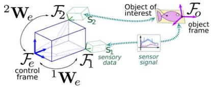
Fig. 1. Multisensor model.
A. Kinematic Model
We consider a robotic system that is equipped withksensors providing data about the robot pose in its environment. The robot joint positions are denotedqand we definen= dim(q). Each sensorSidelivers a signalsiof dimensionmiwithki= 1mi= mand we assumem≥n. A signal component is called a sensor feature. In the case of a motionless environment, the signal time derivative is directly related to the sensor velocityviexpressed
in the sensor frame by
˙
si=Livi (1)
where Li is named the interaction matrix of si [4], [39] and
is of dimensionmi×6. Its analytical form can be derived for many features coming from exteroceptive sensors. It depends mainly on the type of considered sensory data s and on the sensor intrinsic parameters.Limay also depend on other data;
for instance the interaction matrix of an image point that is observed by a camera depends on the depth of that point, which is not actually measured in the image [4].
Now, we consider a reference frameFe in which the robot
velocity can be controlled. This frame can be for instance the end-effector frame for a robot arm as shown in Fig. 1. The screw transformation matrix allows expressing the sensor velocityvi
wrt the robot velocityve
vi=iWeve. (2)
iW
eis given by [38]
iW e=
iR
e ite×iRe 03×3 iRe
(3)
whereiRe∈SO(3)andite ∈R3are, respectively, the rotation matrix and the translation vector betweenFe andFsi.ite×
is the 3×3 skew-symmetric matrix related to ite. Denoting eJ
q∈Rm×n the robot Jacobian, we have
˙
si=LiiWeeJqq.˙ (4)
Denotings= (s1, . . . ,sk)them-dimensional signal of the
mul-tisensor set, (4) allows linking the signal time variation with the joint velocity
˙
with
whereL∈Rm×6k contains the interaction matrices of the sen-sors andWe ∈R6k×6 contains the transformation matrices. In
the following, we assumeJsis of full rankn. We will mention
in Section III-B1 that this assumption could be relaxed, but this paper focuses on the full rank case. We now define the weighted error that will be used in the control law.
B. Weighted Error
The goal of a sensor-based control is to design a control law that makes the robot reach a desired value s∗ of the sensor features. This desired value may be obtained by teaching-by-showing, or through a model at the desired pose; for example in [32], visual servoing is performed with the desired value being the projection of the object model at the desired camera pose.
1) Weighted Error: We define the weighted multisensor sig-nal error as
eH =He (7)
where eis the sensor error defined ase=s−s∗, andHis a diagonal positive semidefinite weighting matrix that depends on the current value ofs. As in all varying-feature-set schemes [31], each componenthi ofHmay vary in order to ensure specific constraints, manage priorities or add or remove a sensor or a feature from the control law. In the case ofksensors,Hyields
H=
whereHiis the weighting matrix for sensorSi.
2) Weighting Canonical Form: Weighting can be performed for several purposes. First, the most simple goal is to balance the disparate sensor contributions during the scheme. As in LQ control, this amounts to optimizing the system behavior by defining a specific weight for each sensor feature. In this paper, we propose also using the weight of a sensor feature to take into account unilateral constraints on that feature. We thus define a generic weighting by
∀i∈[1, m] : hi=hti+hci (9)
where ht
i is tuned for the general balance of the feature, and
wherehc
iallows taking potential constraints into account.
Clas-sical control laws such as visual servo schemes usually use the simplest weighting that corresponds toH=Im, that is
∀i, ht
i = 1andhci = 0. (10)
Each weight(ht
i)imay also be tuned independently, as in LQ
control. In practice, several trials are often necessary to deter-mine the best weighting [44]. In varying-feature-set schemes
Fig. 2. Generic weightinghcfor the basic constraints.
[9], [15], the weights ht
i vary between 0 and 1 depending on
the confidence in each sensor feature. In this paper, we do not focus on the tuning of this weight term, and we setht
i = 1if
the featuresiis always used for the actual navigation task, and
ht
i = 0if the featuresi only corresponds to a constraint to be
ensured. We now explicit the generic formulation for the term
hci handling the constraints.
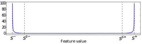
A constraint is usually expressed by an inequality on the value of a sensor feature. This is typically the case for joint limits or image visibility, and is also valid when range sensors are measuring the distance to the obstacles. Singularity avoidance can also be considered by setting a lower bound fordet(J⊤sJs).
In all cases, this corresponds to having to keep the feature value
siin an interval[s−i, s+i ]. In that case, a safe interval[ssi−, ss+i ]
whereρi∈[0,0.5]is a tuning parameter. The weighting termhc i
handling the constraint is then given by
hci =
iis represented in Fig. 2. Similar to a repulsive field [25],
the weight is null in the safe region and continuously increases to∞ as the feature approaches the limit. A constraint is said to be active when its weighthc
i is non-null. The next section
presents the control law and its main properties. In particular, the weights in case of one or several active constraints are studied in Section III-C5.
III. CONTROLLAW
A. Weighted Control Scheme
In the task function approach [39], the task erroretask ∈Rn
is defined by
etask=C(s−s∗) =Ce (13)
whereC∈Rn×m is named the combination matrix and allows us to take into account the redundancy between the sensor fea-tures. A classical controller is then
˙
q=−λetask =−λCe. (14)
A popular choice that tries to ensure an exponential decrease ofetaskisC= ˆJ
+
s, that is an estimation of the Moore–Penrose
pseudo-inverse ofJs. In our case,J+s = (J⊤sJs)−1J⊤s sinceJs
is full rank. This strategy can be seen as a particular case of LQ control [36]. In this framework, a cost functionFhas to be minimized and is defined with
F = (s−s∗)⊤Q(s−s∗) + ˙q⊤Rq˙ (15) whereQandRare weighting matrices that are usually tuned in order to obtain an optimal behavior of the robot. The selection of the elements of Q and R may be computed from a pole placement tuning or considerations on the variance of observed data [44]. In practice, several trials are often necessary to obtain the desired behavior. The corresponding control input yields [26]
This control law is the same as (14) for the particular weighting
Q=Im andR= 0.
When considering the weighted erroreH instead of e, the associated Jacobian isJH =HJs. In this case, control law (14)
yields
˙
q=−λ(HJˆs)+eH =−λ(HJˆs)+He. (17)
The combination matrix ofeis thus given by
C= (HˆJs)+H. (18)
When compared with LQ control, this combination matrix corre-sponds to the particular weightingQ=H2andR= 0. Indeed, in this case the LQ scheme (16) yields
˙
The main difference between our scheme and classical LQ con-trol is about the use of the weighting matrixQ. In LQ control, it is usually tuned in order to obtain an optimal behavior of the robot. In the proposed scheme, we focus on the balance between the different features and sensors and potential constraints. Ac-tually, the two strategies may be used in a complementary way: if bothHandQare defined from their respective frameworks, a global scheme can be designed by using the weighting matrix
H⊤QH. In addition, a control cost matrixR= 0could be used if needed.
As for the estimation of Js, the most popular choices are
summarized in [24], showing the induced behaviors. From (6), computingJsamounts to choosing how to estimate the
interac-tion matricesLiand the transformation matricesiWe.
1) Interaction Matrices: Several possibilities exist for the interaction matrices [4]. Two classical choices are to use the current interaction matrix, or its value at the desired poseL∗. In this case, the interaction matrix is constant. Another popular strategy is the mean interaction matrix1/2(L+L∗), which was recently shown as an approximation of second-order minimiza-tion [41].
2) Transformation Matrices: If the sensors are rigidly at-tached to the effector, then all transformation matrices are con-stant and can usually be estimated in an offline calibration step. In the other case, for instance in eye-to-hand configuration,We
is not constant and the desired valueW∗e depends on the final 3-D pose of the sensors wrt the effector. This pose is generally unknown in sensor-based control. The most plausible choice is thus to estimate the current transformation matrices from the robot geometrical model and calibration.
In the following, we assume that an estimation of the current matricesL andWe is available, which allows us to estimate
Js in real time. We now study the properties of the proposed
scheme.
B. Control Scheme Properties
This section explores the basic properties of the control law. First, we expose the condition for control law continuity and study the case of null weights. We then show local asymptotic stability.
1) Continuity and Influence of Null Weights: The continuity of varying-feature-set control laws has been studied in [31]. In the general case, continuity is ensured under three conditions:
H andJs are continuous and the pseudo-inverse operator is
continuous forHJs. The latter is ensured under the assumption
thatHJs is full rank, which implies in particular that there are
always at leastnnonnull weights. The case of rank change is solved in [31] with a generalized pseudoinverse; however, in this paper we use the classical pseudoinverse and assumeHJs
is full rank. Usual sensor features have a continuous Jacobian
Js. The formulation of the weighting matrix in Section II-B2 is also continuous; hence, the control law is continuous.
Control law (17) is designed to ensure that He˙ =−λHe,
which is different from classical design e˙ =−λe. This dif-ference clearly appears for configurations with null weights. Assuming s= (s1,s0) where features s0 have null weights
precisely, in [16], the combination matrix is defined as C=
The zeroed error components are thus still taken into account and the system behaves exactly as if the desired values for
e0 had been reached, which induces an undesired conservative
behavior to ensure the useless constraints e0= 0. This is not
the case with our approach.
2) Local Asymptotic Stability: Varying-feature-set schemes usually neglect the time variation ofHby assuming the weight-ing matrix is varyweight-ing slowly, or that it is null at the convergence as in region-reaching visual servoing [5]. Actually, whenHis integrated into the combination matrix and assumed to be vary-ing wrt s, the stability analysis is the same as with a varying
Js [4]. As for classical IBVS schemes, a direct consequence
is that global asymptotic stability cannot be proven as soon as redundant features are involved (m > n). From (6) and (18), the task error variation yields
˙
etask =Ce˙+ ˙Ce= (CJs+O) ˙q
=−λ(CJs+O)etask (25)
where O∈Rn×n = 0, when etask = 0 [4]. With the
combi-nation matrix from (18), this scheme is known to be locally asymptotically stable (LAS) in a neighborhood ofe= 0if [18]
CJs = (HJˆs)+HJs>0. (26)
The system is thus LAS, whenHJs andHJˆsare full rank and
when the JacobianJsis sufficiently well estimated, which is the
case in general. In this case, potential local minima correspond to configurations whereH2(s−s∗)∈Ker Jˆs
⊤
. We will see in Section IV-A how to deal with this issue. Let us also note that determining theoretically the convergence domain seems to be out of reach. However, as we will see in Section V, it reveals to be surprisingly large in practice.
C. Particular Case of One Constraint
In this section, we focus on the case where only one active constraint is involved. In that case, we show that a sufficiently high weight induces the decreasing of the corresponding feature error. In particular, we determine the minimal weight ensuring the corresponding constraint is respected. Dealing with several active constraints simultaneously is finally discussed at the end of this section.
1) Sufficient Weight: We assume the reference values∗
iof the
feature si is in the confidence interval. A sufficient condition for the associated constraint to be ensured is that the errorei=
si−s∗
idecreases. We now show that this can be ensured at each
iteration if the associated weight is high enough. A classical Lyapunov function that is associated with the weighted error is
V(eH) = 12e⊤HeH. Assuming that we are in the domain of local
stability, the time derivative ofV yields
˙
The erroreidecreasesiffeiei˙ <0, which is equivalent to
h2
Hence, in any configuration there exists a sufficiently high weighthithat ensures that the corresponding feature error norm is decreasing. Note that ifei˙ = 0orei= 0, then the correspond-ing constraint is de facto ensured.
This property that a sufficient weight exists has been recently highlighted in [21], where the parallel is drawn with the GPM approach and constrained optimization.
Isolating the particular featuresi, the control law (17) can be written as the minimum-norm solution to
min that is related to all features exceptsi. It has been shown in [42] that the solution to (29) whenhitends to infinity is exactly the solution to the constrained minimization
min
Note that (30) corresponds to the GPM approach with featuresi
used as the priority task and the other features as the secondary task. At a given iteration and if the JacobianJi is sufficiently
well estimated, the conditioneiei˙ <0is ensured with the system (30) since in this case,eiei˙ ≈e˙∗
iei=−λe2i <0. Hence, coming
back to (29), there exists a valuehm in
i such that
∀hi> hm ini , eiei˙ <0. (31)
The decrease of the error, and hence the corresponding con-straint, can thus be ensured with a finite weight at any given it-eration. We now explicit the computation of this minimal weight. 2) Minimal Weight: We denotesithe feature corresponding to the considered constraint. The goal here is to disturb the task
eias little as possible by determining the weighthi that is as
small as possible, yet sufficiently high to ensure the correspond-ing constraint.
The time variation of the constrained feature is given by
˙
si=Jiq˙ =−λJi(HJs)+H(s−s∗) (32)
=−λJi(J⊤
sH⊤HJs)−1(J⊤iHi2ei+h2iJ⊤iei). (33)
We now show that ensuringsi˙ = 0leads to a linear condition onh2
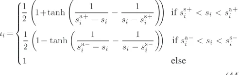
Fig. 3. Activation function for lower and upper bounds.
Fig. 4. Configurations C1 (left) and C2 (right). The feature approaches the nearest limit in C1, while it goes away in C2.
A is an n×n full rank symmetric matrix. The constrained feature time variation thus yields, up to the scale factor λ
D
adjugate matrix properties, the first row of adj(RH2R⊤)does not depend onh1. Thus, asR⊤is lower triangular, the first row of JAdoes not depend onh1, which concludes the demonstration
that can be extended to all indexes.
We denote the twohi-independent scalars
ci=−JiAJ⊤
This leads to two configurations C1 and C2 that are represented in Fig. 4:
1) Approaching the constraint (C1): Ifci andai have the same sign, then the robot is going toward the constraint. In that case there exists a positiveh2
i such thatsi˙ is null.
2) Avoiding the constraint (C2):Ifciandaido not have the same sign, then the robot is moving away from the con-straint; self-avoidance occurs and the avoidance scheme can be ignored.
From this observation, we define the values sa− and sa+
where the feature has to stop
sa−
i =s−i +ρa(s+i −s−i) sa+i =s+i −ρa(s+i −s−i)
(41)
whereρa< ρis a tuning parameter. The minimal value can thus
be computed analytically from (40)
hm ini =
i = 0corresponds to the configurations where
self-avoidance occurs.
Such a minimal weight ensures that the constraint is ensured at least whensi=sa
i since in this case we havesi˙ = 0. However,
as we do not need to ensure the constraint beforesi=sa i, the
minimal weight is smoothly taken into account with an injection function.
3) Injection Function: We address the injection ofhm inwith
the following form of the weights:
∀i, hci =μi(si)hm ini (43)
whereμi(si)∈[0,1]is a continuous function.
To ensure the continuity ofHJs andHe, weights must be
null at feature activation and deactivation, and increasing as the constrained feature values vary from the safe limit to the physical limit. In our case, the injection function is null when
si =ss
whereμiisC∞and smoothly increases the weight as the feature reaches the limit, withμi(sa−
i ) =μi(s a+
i ) = 1andμi(ssi−) = μi(ss+i ) = 0. The proposed injection function is represented in Fig. 3. This allows activating the feature as progressively as possible, hence with the smallest disturbance on the main task.
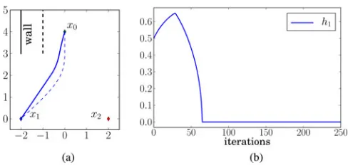
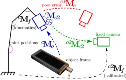
4) Example in Simulation: The proposed minimal weight is illustrated in simulation. The simulation setup is voluntarily simple and consists of a 2-D Cartesian robot that has to reach a point. The task Jacobian is thusI2. The constraint is to keep a
minimum distance to the wall that is present. The simulation is represented in Fig. 5. The robot starts inx0(0,4). The measured
distance to the wall isd= 2, while the desired distance has been set tod∗= 4. The activation values are defined asda = 1and ds = 3. Denotingex the task error anded the error related to
the constraint, the variables from (39) yield
Jx=I2 Jd = [1 0] A=I2 ed =−2. (45)
Fig. 5. Minimal weight in simulation. (a) Robot trajectory and (b) correspond-ing weight. The dotted line shows the trajectory with the generic weight (12). The minimal weight value is 0.5 at the beginning, and then it increases as the robot approaches the wall. The minimal weight is null once the robot has passed the wall. (a) Trajectory tox1. (b) Weight tox1.
Fig. 6. Weights for configuration C1 (upper bound) and C2 (lower bound). In C1 (indicated by the red line), the feature is going toward its limit and a non-null weight has to be used (herehm in=0.5). In C2 (indicated by the green line),
the other features induce the avoidance; hence, the weight can be null in the activation area. If the feature still approaches the limits, the generic weighting hcis used in both cases.
indeed 0.5, and then increases as the robot comes nearer to the wall. This means the weight is not high enough to haved˙= 0at this position, which is the desired behavior as we want the robot to stop approaching the wall only at
da = 1.
2) If the desired position isx2(2,0), then we havec= 2;
self-avoidance occurs, as can be guessed in Fig. 5(a). This also occurs at the end of the task tox1once the wall is passed,
inducing a null weight and a straight line trajectory. 5) Ensuring Several Constraints: In the case of several con-straints having to be ensured simultaneously, coupling terms appear since a system of equations (40) is highly nonlinear. A solution still exists to stop all the endangered constraints (for instanceq˙ = 0is always a solution) but it would be difficult to compute analytically the corresponding set of optimal weights. The minimal weighting (42) can thus be used together with the generic weighting (12). With this strategy, the weighting is minimal in[sa−, sa+]but is still robust to multiple avoidance.
Such a weighting is represented in Fig. 6. We have assumed that C1 holds for the upper bound with an optimal weight of
hm in=0.5 and that C2 holds for the lower bound; hence, the
optimal weight is null. If the feature goes out of [sa−, sa+],
then the generic weighting is used for both bounds. In this case, an endangered constraint will have its weight increased until it reaches a sufficient value, which explains why the generic weighting (12) is not bounded. As the sufficient and minimal weights for one constraint depend on the other constraints [see (28) and (42)], this can lead to a general increasing of the weights corresponding to all the endangered constraints until avoidance.
In the general case, the induced behavior is satisfactory even if it remains possible to define a task under constraints that would be impossible to perform. In such a case, weights cannot be proven to be finite anymore since the system is no more stable and (27) does not hold. Finally, the sole generic weighting may also be used, leading to a less optimal behavior as seen with the dotted trajectory in Fig. 5(a). We now highlight practical issues for the presented system.
IV. POTENTIALISSUES
Three undesired behaviors may be encountered in the pre-sented system. First, as in all sensor-based approaches, local minima may appear as soon as the system is overdetermined, that ism > n. Reaching a desired position where the constraints are active is a second issue. Finally, having potentially high weights may cause oscillations in some cases. In this section, we propose several strategies for each of these issues.
A. Escaping From Local Minima
The main drawback of the proposed scheme, as for all redun-dant reactive sensor-based schemes, is the potential existence of local minima. Indeed, as soon asm > n only local stabil-ity can be proven. As no planning is considered with a higher level controller, the approach that has been investigated is to detect that a local minimum has been reached, and try to escape from it. A local minimum is easily detected as it is necessarily a configuration where the end-effector velocity is almost null, while some of the weighted error components H(s−s∗)are not null. The detection condition can thus be defined by two parametersvǫandeǫsuch as a local minimum corresponds to a configuration where
ve < vǫ and H(s−s∗) > eǫ. (46)
Once a local minimum has been detected, we allow the sys-tem to perform nonoptimal motion in terms of the sensor-based task, by increasing the weights corresponding to the active con-straints. This can be seen as a random walk [2], where we use the structure to compute the escaping motion. We denoteecthe set
of features that regroups the active constraints, andetthe other
features. The corresponding strategy to modify the weighting matrix is described in Algorithm 1; the weightsHc are
Fig. 7. Joint position and weights while escaping from a local minimum. Oscillations appear inh3(indicated by a red line), inducing small oscillations
in the robot motion. (a) Joint positionsq. (b) Joint weightsHq.
configuration where
⎧ ⎪ ⎪ ⎪ ⎨ ⎪ ⎪ ⎪ ⎩
H
c 0
0 Ht
2
(s−s∗)∈ KerˆJ+s
αH
c 0
0 Ht
2
(s−s∗)∈/ KerˆJ+s.
(47)
In this case, the obtained motion is null if α= 1, while it is not with the obtained α >1. This may not be true for any givenαbut in this case Algorithm 1 will carry on increasing
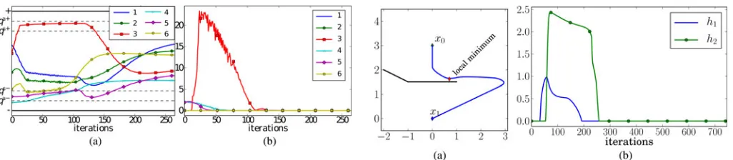
αand eventually lead to a configuration that is out of the null space. Meanwhile, ifαmakes the weights reach very high val-ues, the system is slowed down by the adaptive gain detailed in Section IV-C.αis always equal to 1 as long as no local minimum has been reached. During normal convergence,αis slowly set back to 1. The proposed algorithm makes the active constraints more repulsive, which can be seen as a temporary hierarchy between the active constraints and the other features. Still, such a hierarchy seems natural as constraints have of course to be ensured. On the opposite, going out of a local minimum often prevents us from performing optimally the positioning task, as the escaping motion is usually opposed to the motion that is induced by the task. That is why we temporarily increase the weights of the constraints. The tuning ofα+andα−may be dif-ficult. In practice,αhas to reach a sufficiently high value in order to ensure that the robot will not go back to the same local min-imum. A condition to allow the escape from a local minimum is thatα+α−>1. This corresponds toαincreasing faster than it decreases back to 1. The values we used areα+ =1.05 and α− =0.99. This strategy is inspired by simulated annealing [3], where the parameterαacts as the annealing temperature. We now show two simulation examples of the proposed algorithm. 1) Joint Limits: The induced behavior is represented in Fig. 7 for a simulation of joint limit avoidance in visual ser-voing. A local minimum occurs around iteration 10. We can see in Fig. 7(a) that the joint positions are barely evolving from iter-ation 20 to 70, and that joint limit avoidance is active for joint 3. The joint weights are artificially increased as seen in Fig. 7(b). As the most critical joint isq3, the corresponding weight is far
more important than the others. This allows escaping from the local minimum and induced oscillations are very small in prac-tice. Finally, it is interesting to note that local minima rarely occur wrt the number of features compared with the available DOFs. In particular, in [23], we have performed exhaustive
sim-Fig. 8. Two-Dimensional Cartesian robot escaping from a local minimum. (a) Without the proposed strategy the robot is stuck in the indicated position. (b) The corresponding weights (one per wall) are quickly increasing at the beginning, before slowly decreasing. (a) Trajectory. (b) Weights.
ulations fusing 2-D and 3-D visual servoing. No local minima have been found in this configuration.
2) Two-Dimensional Cartesian Robot: We use the robot setup presented in Section III-C4. Walls are set up such that a local minimum exists, as shown in Fig. 8(a). Without the pro-posed algorithm the robot ends up in the indicated position. The proposed strategy allows the robot escaping the local minimum and uses the structure of the task to find an exit. In Fig. 8(b), we can see that the corresponding weights are quickly increased before slowly decreasing. This illustrates the balance between
α+andα−. Of course, as it is only a reactive scheme some local minima still exist, particularly when the situation is symmetri-cal. Indeed, in this case increasing the weight would only lead to going backward. Complex traps such as U-shapes may not be escaped either; in such cases a planning strategy should be used.
B. Reaching an Unsafe Position
If the desired position is outside the safe area, that is
s∗ ∈]s−, ss−]∪]ss+, s+], the main task cannot be perfectly
per-formed as it does not correspond to the global minimum of the complete weighted task. Indeed, denoting s= (st,sc)where st corresponds to the main task andsc to the constraints, the
desired position is defined by
q∗= arg min q
e⊤tH2tet= arg min
q
e⊤H2e
(48)
wheree⊤H2e=e⊤tH2tet+e⊤cH2cec. A sufficient condition to overcome inequality (48) is to ensure thatHc= 0in a neigh-borhood of the desired position.
To do so, we introduce a progress parameterξ( et )smoothly
making the constraint weights null when the main task gets close to completion
ξ( et )
= ⎧ ⎪ ⎪ ⎪ ⎨ ⎪ ⎪ ⎪ ⎩
0, if et ≤e0
1, if et ≥e1
1 2
1+ tanh
1
e1− et
− 1
et −e0
, else
Fig. 9. Oscillations in a corridor. Without the adaptive gain, the robot oscillates between the two walls (green line). The adaptive gain allows drawing a smooth trajectory (indicated by the dotted blue line).
where e0 and e1 are defined so that the constraints are
to-tally ignored when the main task is close to completion, that is et < e0. The corresponding weighting matrix yields H=Diag(Ht, ξ( et )Hc)and is equal toH∗ =Diag(Ht,0)
in the vicinity of the desired position. The desired position can thus be reached. Finally, depending on the situation, one may or may not use this progress parameter; indeed in some config-urations it is preferable to converge to a compromise between the desired position and the constraints, typically if the desired position lies outside of the boundaries of the constraints.
C. Avoiding Oscillations
The generic weights (12) increase when approaching the con-straints. When several constraints are reached, this may lead to oscillations or even to violating the constraints due to discretiza-tion. In our case, an efficient way to cope with this issue is an adaptive gain depending on H that slows the system in the vicinity of the constraints. The LAS analysis in Section III-B2 is of course still valid with a varying gain, since it can be consid-ered part of the varying combination matrix. The control gainλ
involved in (17) is given by
λ( H ) = (λ0−λ∞)e− λ′
0
λ0−λ∞ H +λ∞ (50)
where
1) λ0 =λ(0)is the gain in 0, that is for very small weights.
2) λ∞= limH →∞λ( H )is the gain to infinity, that is for very high weights.
3) λ′0is the slope ofλat H = 0.
In practice, we have used the valuesλ0 = 1,λ∞ =0.1, and λ′0 =0.5. The proposed strategy is illustrated in simulation in
Fig. 9, with the 2-D Cartesian robot setup. This time the walls draw a corridor. If the gain is too high, oscillations appear (shown by the green line). This is not the case if the adaptive gain is used (shown by the dotted blue line).
Finally, in the case of opposed constraints, hence, several in-creasing weights, such as adaptive gain, would eventually make the robot stop if no solution exists. This seems an acceptable behavior in such a bad situation.
We now present the experimental results that illustrate various aspects of the proposed scheme.
Fig. 10. Experimental setup. (a) Eye-in-hand camera with a 3-D landmark. (b) Observed object. (c) Eye-to-hand camera.
Fig. 11. Integration of various subsystems. Hybrid eye-in-hand features for the visibility constraint, eye-to-hand cooperation, and joint positions to avoid joint limits.
V. EXPERIMENTALRESULTS
In order to illustrate the proposed approach, experiments are carried on a 6-DOF Gantry robot. The control laws are imple-mented using ViSP software [33]. We first detail the experimen-tal setup and its calibration. The sensors and constraints are then introduced one after the other in the control law.
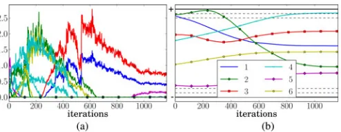
The eye-in-hand camera observes a fixed object, the CAD model of which is known. Its edges are tracked to allow for the pose estimation at camera rate (30 Hz) [8]. The eye-in-hand camera carries a landmark that allows its 3-D tracking in the eye-to-hand view [32]. The carried landmark is composed of 30 dots. Both cameras are calibrated. The pose between the eye-in-hand camera and the landmarkcMo2is roughly calibrated. The
eye-to-hand camera pose wrt the robot reference framefMc2is also
roughly calibrated (see Fig. 11). Fig. 12 represents the two initial images. The robot translation joints 2 and 3 are represented in Fig. 12(b). Joint 2 thus corresponds to a horizontal motion, while joint 3 corresponds to a vertical motion in the eye-to-hand view. The initial and desired poses make it necessary for the robot to move away from the observed object in order to keep it entirely in the field of view (FoV). As we will see, this backward motion makes the end-effector approach not only the upper limit of the eye-to-hand image, but also some joint limits.
Fig. 12. Initial images. (a) The object is large in the eye-in-hand image. (b) Three-dimensional landmark approaches the top of the eye-to-hand image. (a) Eye-in-hand initial image. (b) Eye-to-hand initial image.
Fig. 13. (a) Without the visibility constraint, the observed object leaves the FoV in case 0. (b) Moving landmark leaves the FoV in case 1. (a) Case 0: eye-in-hand image. (b) Case 1: eye-to-hand image.
strategy exposed in Section IV. The adaptive gain (50) is also computed from the activation matrix norm. We now present the system behavior, while the constraints are added one after the other.
A. Pure Position-Based Visual Servo (Case 0)
As previously said, the pose between the eye-in-hand cam-era and the object is estimated at each itcam-eration of the control scheme. It is thus possible to perform position-based visual servo (PBVS) [43].
The corresponding 3-D features ares3d = (c∗tc,c∗θuc). They
describe the transformation between the current and the desired camera pose. The associated desired features is a null vector, and the interaction matrixL3d is known to be block-diagonal,
inducing decoupled translational and rotational motions [4]. In perfect conditions, the corresponding camera trajectory is a 3-D straight line. The associated weighting is classically constant, which corresponds toH3d =I6. Furthermore, this ensures that
the matrixHJsis full rank, which is a condition for the control
law continuity.
The main drawback of PBVS is the lack of control in the image: control is done only in the 3-D space and does not ensure that the observed object stays in the FoV. In our case, this lack of control clearly appears in Fig. 13(a). After few iterations, the object leaves the FoV and the task cannot be performed anymore. We thus add the visibility constraint into the scheme.
Fig. 14. Case 1. (a) The weighting is quite small for the visibility constraint. (b) Joint positions are inside their limits but joint 2 (indicated by the green line) approaches the upper bound. (a) Visibility weightsH2d. (b) Joint positionsq.
B. Adding the Visibility Constraint (Case 1)
The visibility constraint in visual servoing has been previ-ously addressed through switching control law [14], or visual planning [7], [12], [20], [40]. Here, we define a set of 3-D points(ox
1, . . . ,oxp)that are attached to the observed object,
typically the nodes of the CAD model. As the camera posecMo
is estimated in real time, the 2-D coordinates of the projection of the 3-D points can easily be computed together with their depth. The visibility constraint is taken into account by adding the feature vectors2d as the Cartesian coordinates of these 2-D
points. The well-known analytical expression of the interaction matrix of an image point depends both on its image coordinates (x, y) and on its depth Z [4]. The interaction matrix of s2d
can thus be computed in real time. Similarly, the corresponding desired featuress∗2d = (x∗, y∗)are computed from the desired camera posec∗Mo. Let(x−, x+, y−, y+)be the image borders;
a safe region can be defined as in (11). In this experiment, we useρ= 5%. Finally, the feature vector is defined by
s= s
3d
s2d
· · · PBVS (dim. 6)
· · · Visibility (dim. 2×12) (51) where the dimensions of the feature vectors are detailed: six components for the PBVS, and 2×12 for the visibility con-straint (12 nodes in the object CAD model). The corresponding weighting matrix isH=Diag(I6,H2d),whereH2d is derived
from (9) usinght= 0andhc given by (12). We can note that
the global minimum corresponds to the desired pose; indeed, if s3d =s∗3d, then cMo =c∗Mo, and s2d =s∗2d. Hence, the
progress parameter (49) is not used for this constraint, as the robot will converge to the desired pose even if some constraints are active. The resulting images are shown in Fig. 16. The ac-tive nodes are plotted in orange for the visibility constraint. This time the object stays in the FoV during the whole scheme. The visibility weightsH2dare represented in Fig. 14(a). Their value
Fig. 15. Case 2. Visibility constraints in (a) eye-in-hand and (b) eye-to-hand are competing at iteration 240. (c) At this time, joint 2 passes its upper limit. (a) Eye-in-hand weightsH2d. (b) Eye-to-hand weightsHe x t. (c) Joint positionsq.
Fig. 16. Case 2: This time the camera goes to the right of the eye-to-hand image while ensuring the eye-in-hand visibility constraint. (a) Eye-in-hand view (iter. 240). (b) Eye-to-hand view (iter. 240).
Finally, Fig. 13(b) shows that the 3-D landmark goes out of the eye-to-hand view around iteration 240, that is when the camera moves away from the object to keep it in the FoV.
C. Adding the Eye-to-Hand Visibility Constraint (Case 2)
We now take into account the visibility constraint in the eye-to-hand view. The modeling is the same as previously exposed. The considered points are the 30 points from the 3-D landmark. We denotesextthe corresponding 2-D features. The global
fea-ture vector is thuss= (s3d,s2d,sext), and the weighting matrix
isH=Diag(H3d,H2d,Hext),whereHext is defined exactly
asH2d.
The resulting images are shown in Fig. 16. This time, the 3-D landmark stays in the eye-to-hand FoV. The eye-in-hand visibility constraint can still be ensured as the camera moves to the right instead of moving up. As seen in Fig. 15(c), this makes joint 2 (shown by the green line) pass its upper limit (which is not the real limit so that it has been possible to realize this experiment).
The corresponding weights are represented in Fig. 15. Adding a new constraint makes the visibility weightsH2dincrease when
compared with the previous section. Indeed, eye-in-hand and eye-to-hand visibility constraints are competing around iteration 240 which makes the eye-in-hand weights pass 10, while one of the eye-to-hand weights reaches 5. As previously mentioned, the maximum weight is reached around iteration 600 for the visibility constraint.
Fig. 17. Case 3. The camera cannot move to the right anymore when the observed object is large in the eye-in-hand image. (a) This time the 3-D landmark comes toward the eye-to-hand camera while rotating around the optical axis (b). (a) Eye-in-hand view (iter. 240). (b) Eye-to-hand view (iter. 240).
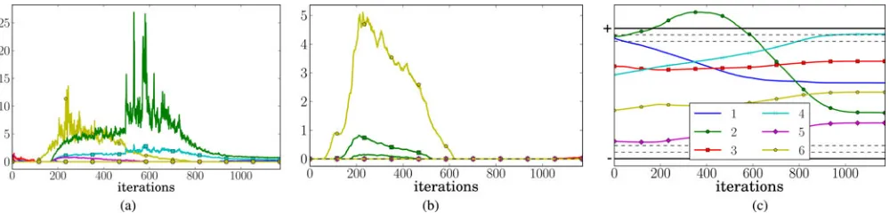
D. Adding the Joint Limit Avoidance (Case 3)
We now take into account the joint positions in the task. The global feature vector yields
s= ⎡ ⎢ ⎢ ⎢ ⎣
s3d
s2d
sext
q
⎤ ⎥ ⎥ ⎥ ⎦
· · · PBVS (dim. 6)
· · · Eye-in-hand visibility (dim.2×12)
· · · Eye-to-hand visibility (dim.2×30)
· · · Joint positions (dim. 6).
(52)
The corresponding weighting matrix is thus H=Diag(H3d, H2d,Hext,Hq), whereHq regroups the joint weights. We use the strategy exposed in Section III-C2;Hq corresponds to the optimal weighting (43). The activation and safe areas are defined withρ=10% and ρa =5%. For this constraint, the progress
parameter (49) is used as the desired position is likely to lie in the joint unsafe area.
Fig. 18. Weights of the different subsystems. (Left) eye-in-hand 2-D points. (Middle) Eye-to-hand 2D points. (Right) Joint positions. All constraints occur around iteration 300, making the weights have significative values. The adaptive gain (shown by a black curve) shows the system slows down at this moment. (a) Eye-in-hand weightsH2d. (b) Eye-to-hand weightsHe x t. (c) Joint weights and adaptive gain.
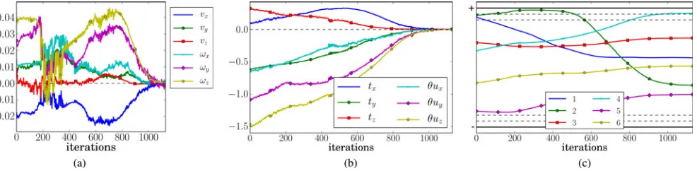
Fig. 19. General behavior of the robot. Camera velocity (left) shows some oscillations when passing the vicinity of all constraints. PBVS error (middle) indicates that the visual servoing is performed during the task. Joint positions (right) highlight the limit being avoided. (a) Camera velocity setpoint. (b) PBVS error. (c) Joint positions.
constraint has some weights reaching 20, while the eye-to-hand and the joint weights reach 5. As previously announced these values are still acceptable and do not endanger the condition-ing ofHand the whole system is stable. Reducing artificially the joint limit would typically lead to a configuration where the task could actually not be performed without violating the constraints and the robot would have stopped at this position.
As previously mentioned, a second peak value is reached for one visibility weight around iteration 600. This time, the corresponding value is less than 10, compared with 25 in case 2. This constraint is thus less endangered by the trajectory from case 3 than the one from case 2. As for the general behavior of the robot, Fig. 19(a) reveals that some oscillations appear in the velocity setpoint. This is due to the high number of constraints that are near to violation at the same time. We can note in Fig. 18(c) that the adaptive gain is reduced by 10 at this time. This is clearly visible in Fig. 19(a) that the system slows down around iteration 240. The measurement of the joint positions in Fig. 19(c) shows that the general motion remains smooth all along the task and, especially, even when joint 2 is near its limit. Finally, Fig. 19(b) represents the PBVS error. Even if the corresponding weighting matrix is the identity, the other weights prevents the PBVS from decreasing exponentially. The convergence is still satisfactory and oscillations are quite small.
E. Comparison Between the Several Cases
Fig. 20 compares the trajectories corresponding to the exper-iments presented. This shows very clearly that the end
effec-Fig. 20. Three-dimensional trajectories for the presented cases, observed from the eye-to-hand camera. Pure PBVS (indicated by the cyan line) begins by a straight line, before getting inconsistent when the tracker loses the object. Case 1 (indicated by the blue line) corresponds to the trajectory that reaches the highest point, as the eye-to-hand visibility is not taken into account. Case 2 (indicated by the green line) makes the camera go to the right instead of going up. Finally, case 3 (indicated by the red line) forces the camera to draw another trajectory in order to ensure all the constraints.
trajectory is a straight line until the failure due to the tracker losing the object. When not using the eye-to-hand image, the camera tends to go up (case 1, indicated by blue). On the op-posite, the runs that use the eye-to-hand camera share a lower trajectory. In particular, the camera going right instead of going up is clearly visible for case 2 (shown by the green line). We highlight that no local minimum is reached for any combina-tion of features. The implicit concurrency allows adding new constraints without having to model the potential coupling.
F. Other Experiments
The presented experiment illustrates the general properties of our approach. In complementary works, we have also high-lighted specific aspects through other types of experiments. In particular, exhaustive simulations have been carried out for the visibility constraint (see case 1). We have simulated 9900 ser-voings, that is a large set of combinations for 100 initial and final poses, showing that 98% converge while ensuring the vis-ibility constraint with the maximum weight being less than 20. The other cases converge with higher weights, or with a smaller control gain. In [23], our approach has also been compared with other control laws that address the visibility constraint. The joint limit avoidance has been validated in [22] on a six-DOF robot arm Adept Viper850 for several positioning tasks in visual servoing. Finally, the proposed framework has also been used in ultrasound images in [27], to maintain the visibility of an anatomic element of interest during tele-echography.
VI. CONCLUSION
This paper has proposed a generic approach to multisensor and multiconstraint fusion in sensor-based control. The litera-ture classically addresses this issue by a hierarchical approach or by performing a weighted mean of the velocities that are com-puted for each task. We proposed performing the data fusion at the level of the features, by introducing a dynamic weighting matrix. While some tuning aspects are similar to LQ control, activation and deactivation of the features is part of the varying-feature-set approach, which has been recently formalized for one sensor [31]. The general idea is that a robotic system can handle a high-dimensional task and several constraints without having to explicit the hierarchy or perform a manual tuning of the feature weights. The main properties of the proposed control law have been exposed, concurring to the classical conditions on the system rank with local asymptotic stability and potential local minima in the case of redundancy. The scheme is generic even for sensors that are not rigidly attached to the end-effector frame. The main drawbacks of the proposed scheme are related to its nature being only reactive. The additional strategies that are proposed for the particular cases of local minima and un-safe desired position both consist in modifying the activation matrix independently from its initial design in terms of sub-system integration. This can be viewed as the beginning of a higher level controller that takes into account the global config-uration and balances the weighting matrix so that the induced trajectory avoids or escapes local minima. The versatility of the approach has been illustrated by considering a multisensor
multiconstraint task. Several experiments have shown that the proposed approach can handle various combinations of sensors and constraints for a positioning task. Future work will consist in extending this framework to other types of sensors such as laser range or haptic devices. Other strategies, such as relaxing some constraints, could also increase the convergence domain of the proposed scheme. This could be suitable, for instance, for the visibility constraint, where some parts of the object could be allowed to leave the field of view.
ACKNOWLEDGMENT
The authors would like to acknowledge P.-B. Wieber for his valuable feedback on this study.
REFERENCES
[1] G. Allibert, E. Courtial, and F. Chaumette, “Predictive control for con-strained image-based visual servoing,”IEEE Trans. Robot., vol. 26, no. 5, pp. 933–939, Oct. 2010.
[2] J. Barraquand and J. Latombe, “Robot motion planning: A distributed representation approach,”Int. J. Robot. Res., vol. 10, no. 6, pp. 628–649, 1991.
[3] S. Brooks and B. Morgan, “Optimization using simulated annealing,”The Statistician, vol. 44, no. 2, pp. 241–257, 1995.
[4] F. Chaumette and S. Hutchinson, “Visual servo control—Part I: Basic approaches,”IEEE Robot. Autom. Mag., vol. 13, no. 4, pp. 82–90, Dec. 2006.
[5] C. Cheah, D. Wang, and Y. Sun, “Region-reaching control of robots,”
IEEE Trans. Robot., vol. 23, no. 6, pp. 1260–1264, Dec. 2007.
[6] G. Chesi, “Visual servoing path planning via homogeneous forms and LMI optimizations,”IEEE Trans. Robot., vol. 25, no. 2, pp. 281–291, Apr. 2009.
[7] G. Chesi and Y. Hung, “Global path-planning for constrained and optimal visual servoing,”IEEE Trans. Robot., vol. 23, no. 5, pp. 1050–1060, Oct. 2007.
[8] A. Comport, E. Marchand, and F. Chaumette, “Efficient model-based tracking for robot vision,”Adv. Robot., vol. 19, no. 10, pp. 1097–1113, Oct. 2005.
[9] A. Comport, E. Marchand, and F. Chaumette, “Statistically robust 2-D visual servoing,”IEEE Trans. Robot., vol. 22, no. 2, pp. 415–420, Apr. 2006.
[10] P. Danes and D. Bellot, “Towards an LMI approach to multicriteria visual servoing in robotics,”Eur. J. Control, vol. 12, no. 1, pp. 86–110, 2006. [11] W. Decr´e, R. Smits, H. Bruyninckx, and J. De Schutter, “Extending iTaSC
to support inequality constraints and non-instantaneous task specifica-tion,” inProc. IEEE Int. Conf. Robot. Autom., 2009, pp. 964–971. [12] L. Deng, F. Janabi-Sharifi, and W. Wilson, “Hybrid motion control and
planning strategies for visual servoing,” IEEE Trans. Ind. Electron., vol. 52, no. 4, pp. 1024–1040, Aug. 2005.
[13] F. Fahimi, C. Nataraj, and H. Ashrafiuon, “Real-time obstacle avoidance for multiple mobile robots,”Robotica, vol. 27, no. 2, pp. 189–198, Mar. 2009.
[14] N. Gans and S. Hutchinson, “Stable visual servoing through hybrid switched-system control,”IEEE Trans. Robot., vol. 23, no. 3, pp. 530–540, Jun. 2007.
[15] N. Garc´ıa-Aracil, E. Malis, R. Aracil-Santonja, and C. P´erez-Vidal, “Con-tinuous visual servoing despite the changes of visibility in image features,”
IEEE Trans. Robot., vol. 21, no. 6, pp. 1214–1220, Dec. 2005.
[16] A. Hafez and C. Jawahar, “Visual servoing by optimization of a 2-D/3-D hybrid objective function,” inProc. IEEE Int. Conf. Robot. Autom., Rome, Italy, 2007, pp. 1691–1696.
[17] K. Hosoda, K. Igarashi, and M. Asada, “Adaptive hybrid control for visual and force servoing in an unknown environment,”IEEE Robot. Autom. Mag., vol. 5, no. 4, pp. 39–43, Dec. 1998.
[18] A. Isidori,Nonlinear Control Systems. New York, NY, USA: Springer-Verlag, 1995.
[20] M. Kazemi, M. Mehrandezh, and K. Gupta, “Kinodynamic planning for visual servoing,” inProc. IEEE Int. Conf. Robot. Autom., 2011, pp. 2478– 2484.
[21] F. Keith, P. Wieber, N. Mansard, and A. Kheddar, “Analysis of the discon-tinuities in prioritized tasks-space control under discreet task scheduling operations,” presented at IEEE Int. Conf. Intelligent Robots System, San Francisco, CA, USA, Sep. 2011.
[22] O. Kermorgant and F. Chaumette, “Avoiding joint limits with a low-level fusion scheme,” inProc. IEEE/RSJ Int. Conf. Intell. Robots Syst., San Francisco, CA, USA, Sep. 2011, pp. 768–773.
[23] O. Kermorgant and F. Chaumette, “Combining IBVS and PBVS to ensure the visibility constraint,” inProc. IEEE/RSJ Int. Conf. Intell. Robots Syst., San Francisco, CA, USA, Sep. 2011, pp. 2849–2854.
[24] O. Kermorgant and F. Chaumette, “Multi-sensor data fusion in sensor-based control: Application to multi-camera visual servoing,” in Proc. IEEE Int. Conf. Robot. Autom., Shanghai, China, May 2011, pp. 4518– 4523.
[25] O. Khatib, “Real-time obstacle avoidance for manipulators and mobile robots,”Int. J. Robot. Res., vol. 5, no. 1, pp. 90–98, 1986.
[26] F. Lewis and V. Syrmos,Optimal Control. New York, NY, USA: Wiley-Interscience, 1995.
[27] T. Li, O. Kermorgant, and A. Krupa, “Maintaining visibility constraints during tele-echography with ultrasound visual servoing,” inProc. IEEE Int. Conf. Robot. Autom., Saint Paul, MN, USA, May 2012, pp. 4856– 4861.
[28] E. Malis, G. Morel, and F. Chaumette, “Robot Control Using Disparate Multiple Sensors,”Int. J. Robot. Res., vol. 20, no. 5, pp. 364–377, May 2001.
[29] N. Mansard and F. Chaumette, “Task sequencing for sensor-based con-trol,”IEEE Trans. Robot., vol. 23, no. 1, pp. 60–72, Feb. 2007. [30] N. Mansard, O. Khatib, and A. Kheddar, “A unified approach to integrate
unilateral constraints in the stack of tasks,”IEEE Trans. Robot., vol. 25, no. 3, pp. 670–685, Jun. 2009.
[31] N. Mansard, A. Remazeilles, and F. Chaumette, “Continuity of varying-feature-set control laws,”IEEE Trans. Autom. Control, vol. 54, no. 11, pp. 2493–2505, Nov. 2009.
[32] E. Marchand, F. Chaumette, F. Spindler, and M. Perrier, “Controlling an uninstrumented manipulator by visual servoing,”Int. J. Robot. Res., vol. 21, no. 7, pp. 635–647, 2002.
[33] E. Marchand, F. Spindler, and F. Chaumette, “ViSP for visual servoing: A generic software platform with a wide class of robot control skills,”IEEE Robot. Autom. Mag., vol. 12, no. 4, pp. 40–52, Dec. 2005.
[34] M. Marey and F. Chaumette, “A new large projection operator for the redundancy framework,” inProc. IEEE Int. Conf. Robot. Autom., Anchor-age, AK, USA, May 2010, pp. 3727–3732.
[35] Y. Mezouar and F. Chaumette, “Design and tracking of desirable trajec-tories in the image space by integrating mechanical and visibility con-straints,” inProc. IEEE Int. Conf. Robot. Autom., 2001, vol. 1, pp. 731– 736.
[36] B. Nelson and P. Khosla, “Strategies for increasing the tracking region of an eye-in-hand system by singularity and joint limit avoidance,”Int. J. Robot. Res., vol. 14, no. 3, pp. 418–423, 1995.
[37] N. Papanikolopoulos, P. Khosla, and T. Kanade, “Visual tracking of a moving target by a camera mounted on a robot: A combination of control and vision,”IEEE Trans. Robot. Autom., vol. 9, no. 1, pp. 14–35, Feb. 1993.
[38] R. Paul,Robot Manipulators: Mathematics, Programming, and Control: The Computer Control of Robot Manipulators. Cambridge, MA, USA: MIT Press, 1981.
[39] C. Samson, M. Le Borgne, and B. Espiau,Robot Control: The Task Func-tion Approach. Oxford, U.K.: Clarendon, 1991.
[40] F. Schramm and G. Morel, “Ensuring visibility in calibration-free path planning for image-based visual servoing,”IEEE Trans. Robot., vol. 22, no. 4, pp. 848–854, Aug. 2006.
[41] O. Tahri and Y. Mezouar, “On visual servoing based on efficient second order minimization,”Robot. Auton. Syst., vol. 58, no. 5, pp. 712–719, 2009.
[42] C. Van Loan, “On the method of weighting for equality-constrained least-squares problems,”SIAM J. Numer. Anal., vol. 22, pp. 851–864, 1985. [43] W. Wilson, W. Hulls, and G. Bell, “Relative end-effector control using
cartesian position based visual servoing,”IEEE Trans. Robot. Autom., vol. 12, no. 5, pp. 684–696, Oct. 1996.
[44] B. Wittenmark, R. Evans, and Y. Soh, “Constrained pole-placement using transformation and LQ-design* 1,”Automatica, vol. 23, no. 6, pp. 767– 769, 1987.
[45] T. Yoshikawa, “Basic optimization methods of redundant manipulators,”
Lab. Robot. Autom., vol. 8, no. 1, pp. 49–60, 1996.
Olivier Kermorgantreceived the Graduation de-gree from ´Ecole Centrale Paris, Grande Voie des Vi-gnes, France, in 2004 and the Ph.D. degree in signal processing from the University of Rennes, Rennes, France in 2011.
From 2008 to 2011, he was with the Lagadic Group at Inria Rennes, France. For two years, he was a Research Engineer with the Measurement and Con-trol Department, Arcelor Research, Metz, France. He then joined the Ocean Systems Laboratory, Heriot-Watt University, Edinburgh, U.K., as a Research As-sistant. Since 2012, he has been an Assistant Professor with the University of Strasbourg, Strasbourg, France. His research interests include sensor-based robot control, disturbance rejection, and optimization.
Franc¸ois Chaumettereceived the Graduation de-gree from ´Ecole Nationale Sup´erieure de M´ecanique, Nantes, France, in 1987. He received the Ph.D. degree in computer science from the University of Rennes, Rennes, France, in 1990.
Since 1990, he has been with Inria Rennes, where he is currently a Senior Research Sci-entist and the Head of the Lagadic Group. His research interests include robotics and com-puter vision, especially visual servoing and active perception.