Data Mining:
Concepts and Techniques
Chapter 3: Data Warehousing and
OLAP Technology: An Overview
What is a data warehouse?
A multi-dimensional data model
Data warehouse architecture
Data warehouse implementation
What is Data Warehouse?
Defined in many different ways, but not rigorously.
A decision support database that is maintained separately from
the organization’s operational database
Support information processing by providing a solid platform of
consolidated, historical data for analysis.
“A data warehouse is a subject-oriented, integrated, time-variant,
and nonvolatile collection of data in support of management’s decision-making process.”—W. H. Inmon
Data warehousing:
Data Warehouse—Subject-Oriented
Organized around major subjects, such as
customer,
product, sales
Focusing on the modeling and analysis of data for
decision makers, not on daily operations or transaction
processing
Provide
a simple and concise
view around particular
Data Warehouse—Integrated
Constructed by integrating multiple, heterogeneous data
sources
relational databases, flat files, on-line transaction
records
Data cleaning and data integration techniques are
applied.
Ensure consistency in naming conventions, encoding
structures, attribute measures, etc. among different
data sources
E.g., Hotel price: currency, tax, breakfast covered, etc.
When data is moved to the warehouse, it is
Data Warehouse—Time Variant
The time horizon for the data warehouse is significantly
longer than that of operational systems
Operational database: current value data
Data warehouse data: provide information from a
historical perspective (e.g., past 5-10 years)
Every key structure in the data warehouse
Contains an element of time, explicitly or implicitly
But the key of operational data may or may not
Data Warehouse—Nonvolatile
A
physically separate store
of data transformed from the
operational environment
Operational
update of data does not occur
in the data
warehouse environment
Does not require transaction processing, recovery,
and concurrency control mechanisms
Requires only two operations in data accessing:
Data Warehouse vs. Heterogeneous DBMS
Traditional heterogeneous DB integration: A query driven approach
Build wrappers/mediators on top of heterogeneous databases When a query is posed to a client site, a meta-dictionary is used
to translate the query into queries appropriate for individual
heterogeneous sites involved, and the results are integrated into a global answer set
Complex information filtering, compete for resources
Data warehouse: update-driven, high performance
Information from heterogeneous sources is integrated in advance
Data Warehouse vs. Operational DBMS
OLTP (on-line transaction processing)
Major task of traditional relational DBMS
Day-to-day operations: purchasing, inventory, banking,
manufacturing, payroll, registration, accounting, etc.
OLAP (on-line analytical processing)
Major task of data warehouse system Data analysis and decision making
Distinct features (OLTP vs. OLAP):
User and system orientation: customer vs. market
Data contents: current, detailed vs. historical, consolidated Database design: ER + application vs. star + subject
View: current, local vs. evolutionary, integrated
OLTP vs. OLAP
OLTP OLAP
users clerk, IT professional knowledge worker
function day to day operations decision support
DB design application-oriented subject-oriented
data current, up-to-date detailed, flat relational isolated
historical,
summarized, multidimensional integrated, consolidated
usage repetitive ad-hoc
access read/write
index/hash on prim. key
lots of scans
unit of work short, simple transaction complex query
# records accessed tens millions
#users thousands hundreds
DB size 100MB-GB 100GB-TB
Why Separate Data Warehouse?
High performance for both systems
DBMS— tuned for OLTP: access methods, indexing, concurrency
control, recovery
Warehouse—tuned for OLAP: complex OLAP queries,
multidimensional view, consolidation
Different functions and different data:
missing data: Decision support requires historical data which
operational DBs do not typically maintain
data consolidation: DS requires consolidation (aggregation,
summarization) of data from heterogeneous sources
data quality: different sources typically use inconsistent data
representations, codes and formats which have to be reconciled
Chapter 3: Data Warehousing and
OLAP Technology: An Overview
What is a data warehouse?
A multi-dimensional data model
Data warehouse architecture
Data warehouse implementation
From Tables and Spreadsheets to Data Cubes
A data warehouse is based on a multidimensional data model which views data in the form of a data cube
A data cube, such as sales, allows data to be modeled and viewed in multiple dimensions
Dimension tables, such as item (item_name, brand, type), or
time(day, week, month, quarter, year)
Fact table contains measures (such as dollars_sold) and keys to
each of the related dimension tables
In data warehousing literature, an n-D base cube is called a base
Cube: A Lattice of Cuboids
time,item
time,item,location
time, item, location, supplier all
time item location supplier
time,location
time,supplier
item,location
item,supplier
location,supplier
time,item,supplier
time,location,supplier
item,location,supplier
0-D(apex) cuboid
1-D cuboids
2-D cuboids
3-D cuboids
Conceptual Modeling of Data Warehouses
Modeling data warehouses: dimensions & measures
Star schema
:
A fact table in the middle connected to a
set of dimension tables
Snowflake schema
:
A refinement of star schema
where some dimensional hierarchy is
normalized
into a
set of smaller dimension tables
, forming a shape
similar to snowflake
Fact constellations
:
Multiple fact tables share
Example of Star Schema
time_key day day_of_the_week month quarter year time location_key street city state_or_province country location Sales Fact TableExample of Snowflake Schema
time_key day day_of_the_week month quarter year time location_key street city_key location Sales Fact TableExample of Fact Constellation
time_key day day_of_the_week month quarter year time location_key street city province_or_state country location Sales Fact Tabletime_key item_key branch_key location_key units_sold dollars_sold avg_sales Measures item_key item_name brand type supplier_type item branch_key branch_name branch_type branch
Shipping Fact Table
Cube Definition Syntax (BNF) in DMQL
Cube Definition (Fact Table)
define cube
<cube_name> [<dimension_list>]:
<measure_list>
Dimension Definition (Dimension Table)
define dimension
<dimension_name>
as
(<attribute_or_subdimension_list>)
Special Case (Shared Dimension Tables)
First time as “cube definition”
define dimension
<dimension_name>
as
<dimension_name_first_time>
in cube
Defining Star Schema in DMQL
define cube
sales_star [time, item, branch, location]:
dollars_sold = sum(sales_in_dollars), avg_sales =
avg(sales_in_dollars), units_sold = count(*)
define dimension
time
as
(time_key, day, day_of_week,
month, quarter, year)
define dimension
item
as
(item_key, item_name, brand,
type, supplier_type)
define dimension
branch
as
(branch_key, branch_name,
branch_type)
Defining Snowflake Schema in DMQL
define cube sales_snowflake [time, item, branch, location]:
dollars_sold = sum(sales_in_dollars), avg_sales = avg(sales_in_dollars), units_sold = count(*)
define dimension time as (time_key, day, day_of_week, month, quarter, year)
define dimension item as (item_key, item_name, brand, type, supplier(supplier_key, supplier_type))
define dimension branch as (branch_key, branch_name, branch_type)
Defining Fact Constellation in DMQL
define cube sales [time, item, branch, location]:
dollars_sold = sum(sales_in_dollars), avg_sales = avg(sales_in_dollars), units_sold = count(*)
define dimension time as (time_key, day, day_of_week, month, quarter, year)
define dimension item as (item_key, item_name, brand, type, supplier_type)
define dimension branch as (branch_key, branch_name, branch_type)
define dimension location as (location_key, street, city, province_or_state, country)
define cube shipping [time, item, shipper, from_location, to_location]:
dollar_cost = sum(cost_in_dollars), unit_shipped = count(*)
define dimension time as time in cube sales
define dimension item as item in cube sales
define dimension shipper as (shipper_key, shipper_name, location as location
in cube sales, shipper_type)
define dimension from_location as location in cube sales
Measures of Data Cube: Three Categories
Distributive
: if the result derived by applying the function to
n
aggregate values is the same as that derived by applying
the function on all the data without partitioning
E.g., count(), sum(), min(), max()
Algebraic
:
if it can be computed by an algebraic function
with
M
arguments (where
M
is a bounded integer), each of
which is obtained by applying a distributive aggregate
function
E.g., avg(), min_N(), standard_deviation()
Holistic:
if there is no constant bound on the storage size
needed to describe a subaggregate.
View of Warehouses and Hierarchies
Specification of hierarchies
Schema hierarchy
day < {month <
quarter; week} < year
Set_grouping hierarchy
Multidimensional Data
Sales volume as a function of product, month,
and region
P
ro
du
ct
Re
gi
on
Month
Dimensions: Product, Location, Time Hierarchical summarization paths
Industry Region Year
Category Country Quarter
Product City Month Week
A Sample Data Cube
Total annual sales of TV in U.S.A.
Date
Pr
od
uc
t
C
ou
n
tr
y
sum
sum
TV
VCRPC
1Qtr 2Qtr 3Qtr 4Qtr
U.S.A
Canada
Mexico
Cuboids Corresponding to the Cube
all
product date country
product,date product,country date, country
product, date, country
0-D(apex) cuboid
1-D cuboids
2-D cuboids
Browsing a Data Cube
Visualization
OLAP capabilities
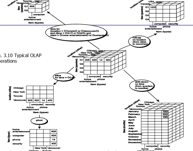
Typical OLAP Operations
Roll up (drill-up): summarize data
by climbing up hierarchy or by dimension reduction
Drill down (roll down): reverse of roll-up
from higher level summary to lower level summary or
detailed data, or introducing new dimensions
Slice and dice:
project and select
Pivot (rotate):
reorient the cube, visualization, 3D to series of 2D planes
Other operations
drill across:
involving (across) more than one fact table
drill through:
through the bottom level of the cube to its
A Star-Net Query Model
Shipping Method AIR-EXPRESS TRUCK ORDER Customer Orders CONTRACTS Customer Product PRODUCT GROUP PRODUCT LINE PRODUCT ITEM SALES PERSON DISTRICT DIVISION CITY COUNTRY REGION Location DAILY QTRLY ANNUALY TimeChapter 3: Data Warehousing and
OLAP Technology: An Overview
What is a data warehouse?
A multi-dimensional data model
Data warehouse architecture
Data warehouse implementation
Design of Data Warehouse: A Business
Analysis Framework
Four views regarding the design of a data warehouse
Top-down view
allows selection of the relevant information necessary for the data warehouse
Data source view
exposes the information being captured, stored, and managed by operational systems
Data warehouse view
consists of fact tables and dimension tables
Business query view
Data Warehouse Design Process
Top-down, bottom-up approaches or a combination of both
Top-down: Starts with overall design and planning (mature) Bottom-up: Starts with experiments and prototypes (rapid)
From software engineering point of view
Waterfall: structured and systematic analysis at each step before
proceeding to the next
Spiral: rapid generation of increasingly functional systems, short
turn around time, quick turn around
Typical data warehouse design process
Data Warehouse: A Multi-Tiered Architecture
Data Warehouse: A Multi-Tiered Architecture
Data
Warehouse
Extract Transform Load RefreshOLAP Engine
Analysis
Query
Reports
Data mining
Monitor & Integrator MetadataData Sources
Front-End Tools
Three Data Warehouse Models
Enterprise warehouse
collects all of the information about subjects spanning
the entire organization
Data Mart
a subset of corporate-wide data that is of value to a
specific groups of users. Its scope is confined to specific,
selected groups, such as marketing data mart
Independent vs. dependent (directly from warehouse) data mart
Virtual warehouse
A set of views over operational databases
Only some of the possible summary views may be
Data Warehouse Development:
A Recommended Approach
Define a high-level corporate data model
Data
Mart
Data
Mart
Distributed
Data Marts
Multi-Tier Data
Warehouse
Enterprise
Data
Warehouse
Data Warehouse Back-End Tools and Utilities
Data extraction
get data from multiple, heterogeneous, and external
sources
Data cleaning
detect errors in the data and rectify them when possible
Data transformation
convert data from legacy or host format to warehouse
format
Load
sort, summarize, consolidate, compute views, check
integrity, and build indicies and partitions
Refresh
propagate the updates from the data sources to the
Metadata Repository
Meta data is the data defining warehouse objects. It stores:
Description of the structure of the data warehouse
schema, view, dimensions, hierarchies, derived data defn, data mart
locations and contents
Operational meta-data
data lineage (history of migrated data and transformation path),
currency of data (active, archived, or purged), monitoring
information (warehouse usage statistics, error reports, audit trails)
The algorithms used for summarization
The mapping from operational environment to the data warehouse
Data related to system performance
warehouse schema, view and derived data definitions
Business data
OLAP Server Architectures
Relational OLAP (ROLAP)
Use relational or extended-relational DBMS to store and manage
warehouse data and OLAP middle ware
Include optimization of DBMS backend, implementation of
aggregation navigation logic, and additional tools and services
Greater scalability
Multidimensional OLAP (MOLAP)
Sparse array-based multidimensional storage engine Fast indexing to pre-computed summarized data
Hybrid OLAP (HOLAP) (e.g., Microsoft SQLServer)
Flexibility, e.g., low level: relational, high-level: array
Specialized SQL servers (e.g., Redbricks)
Chapter 3: Data Warehousing and
OLAP Technology: An Overview
What is a data warehouse?
A multi-dimensional data model
Data warehouse architecture
Data warehouse implementation
Efficient Data Cube Computation
Data cube can be viewed as a lattice of cuboids
The bottom-most cuboid is the base cuboid
The top-most cuboid (apex) contains only one cell
How many cuboids in an n-dimensional cube with L
levels?
Materialization of data cube
Materialize every (cuboid) (full materialization), none (no
materialization), or
some (partial materialization)
Selection of which cuboids to materialize
Based on size, sharing, access frequency, etc.
) 1 1(
n
Cube Operation
Cube definition and computation in DMQL
define cube sales[item, city, year]: sum(sales_in_dollars)
compute cube sales
Transform it into a SQL-like language (with a new operator
cube by, introduced by Gray et al.’96)
SELECT item, city, year, SUM (amount) FROM SALES
CUBE BY item, city, year
Need compute the following Group-Bys
(date, product, customer),
(date,product),(date, customer), (product, customer), (date), (product), (customer)
()
(item) (city)
()
(year)
(city, item) (city, year) (item, year)
Iceberg Cube
Computing only the cuboid cells whose count or
other aggregates satisfying the condition like
HAVING COUNT(*) >=
minsup
Motivation
Only a small portion of cube cells may be “above the
water’’ in a sparse cube
Only calculate “interesting” cells—data above certain
threshold
Avoid explosive growth of the cube
Indexing OLAP Data: Bitmap Index
Index on a particular column
Each value in the column has a bit vector: bit-op is fast The length of the bit vector: # of records in the base table
The i-th bit is set if the i-th row of the base table has the value for
the indexed column
not suitable for high cardinality domains
Cust Region Type
C1 Asia Retail C2 Europe Dealer C3 Asia Dealer C4 America Retail C5 Europe Dealer
RecID Retail Dealer
1 1 0
2 0 1
3 0 1
4 1 0
5 0 1
RecID Asia Europe Am erica
1 1 0 0
2 0 1 0
3 1 0 0
4 0 0 1
5 0 1 0
Indexing OLAP Data: Join Indices
Join index: JI(R-id, S-id) where R (R-id, …) S
(S-id, …)
Traditional indices map the values to a list of
record ids
It materializes relational join in JI file and
speeds up relational join
In data warehouses, join index relates the values
of the dimensions of a start schema to rows in the fact table.
E.g. fact table: Sales and two dimensions city
and product
A join index on city maintains for each distinct city a list of R-IDs of the tuples recording the Sales in the city
Efficient Processing OLAP Queries
Determine which operations should be performed on the available cuboids
Transform drill, roll, etc. into corresponding SQL and/or OLAP operations,
e.g., dice = selection + projection
Determine which materialized cuboid(s) should be selected for OLAP op.
Let the query to be processed be on {brand, province_or_state} with the
condition “year = 2004”, and there are 4 materialized cuboids available: 1) {year, item_name, city}
2) {year, brand, country}
3) {year, brand, province_or_state}
4) {item_name, province_or_state} where year = 2004 Which should be selected to process the query?
Chapter 3: Data Warehousing and
OLAP Technology: An Overview
What is a data warehouse?
A multi-dimensional data model
Data warehouse architecture
Data warehouse implementation
Data Warehouse Usage
Three kinds of data warehouse applications
Information processing
supports querying, basic statistical analysis, and reporting using crosstabs, tables, charts and graphs
Analytical processing
multidimensional analysis of data warehouse data
supports basic OLAP operations, slice-dice, drilling, pivoting
Data mining
knowledge discovery from hidden patterns
supports associations, constructing analytical models,
From On-Line Analytical Processing (OLAP)
to On Line Analytical Mining (OLAM)
Why online analytical mining?
High quality of data in data warehouses
DW contains integrated, consistent, cleaned data
Available information processing structure surrounding
data warehouses
ODBC, OLEDB, Web accessing, service facilities,
reporting and OLAP tools
OLAP-based exploratory data analysis
Mining with drilling, dicing, pivoting, etc.
On-line selection of data mining functions
Integration and swapping of multiple mining
An OLAM System Architecture
Data Warehouse Meta DataMDDB
OLAM
Engine
OLAP
Engine
User GUI API
Data Cube API
Database API Data cleaning Layer3 OLAP/OLAM Layer2 MDDB Layer1 Data Layer4 User Interface Filtering&Integration Filtering Databases
Chapter 3: Data Warehousing and
OLAP Technology: An Overview
What is a data warehouse?
A multi-dimensional data model
Data warehouse architecture
Data warehouse implementation
From data warehousing to data mining
Summary: Data Warehouse and OLAP Technology
Why data warehousing?
A multi-dimensional model of a data warehouse
Star schema, snowflake schema, fact constellations A data cube consists of dimensions & measures
OLAP operations: drilling, rolling, slicing, dicing and pivoting Data warehouse architecture
OLAP servers: ROLAP, MOLAP, HOLAP Efficient computation of data cubes
Partial vs. full vs. no materialization
Indexing OALP data: Bitmap index and join index OLAP query processing
References (I)
S. Agarwal, R. Agrawal, P. M. Deshpande, A. Gupta, J. F. Naughton, R. Ramakrishnan, and S. Sarawagi. On the computation of multidimensional aggregates. VLDB’96
D. Agrawal, A. E. Abbadi, A. Singh, and T. Yurek. Efficient view maintenance in data warehouses. SIGMOD’97
R. Agrawal, A. Gupta, and S. Sarawagi. Modeling multidimensional databases. ICDE’97 S. Chaudhuri and U. Dayal. An overview of data warehousing and OLAP technology.
ACM SIGMOD Record, 26:65-74, 1997
E. F. Codd, S. B. Codd, and C. T. Salley. Beyond decision support. Computer World, 27, July 1993.
J. Gray, et al. Data cube: A relational aggregation operator generalizing group-by, cross-tab and sub-totals. Data Mining and Knowledge Discovery, 1:29-54, 1997.
A. Gupta and I. S. Mumick. Materialized Views: Techniques, Implementations, and Applications. MIT Press, 1999.
J. Han. Towards on-line analytical mining in large databases. ACM SIGMOD Record, 27:97-107, 1998.
References (II)
C. Imhoff, N. Galemmo, and J. G. Geiger. Mastering Data Warehouse Design: Relational
and Dimensional Techniques. John Wiley, 2003
W. H. Inmon. Building the Data Warehouse. John Wiley, 1996
R. Kimball and M. Ross. The Data Warehouse Toolkit: The Complete Guide to Dimensional
Modeling. 2ed. John Wiley, 2002
P. O'Neil and D. Quass. Improved query performance with variant indexes. SIGMOD'97
Microsoft. OLEDB for OLAP programmer's reference version 1.0. In http://
www.microsoft.com/data/oledb/olap, 1998
A. Shoshani. OLAP and statistical databases: Similarities and differences. PODS’00.
S. Sarawagi and M. Stonebraker. Efficient organization of large multidimensional arrays.
ICDE'94
OLAP council. MDAPI specification version 2.0. In http://www.olapcouncil.org/research/
apily.htm, 1998
E. Thomsen. OLAP Solutions: Building Multidimensional Information Systems. John Wiley,
1997
P. Valduriez. Join indices. ACM Trans. Database Systems, 12:218-246, 1987.