Pattern Fabric Defect Detection Using
Nonparametric Regression
S. Halim1
1
Faculty of Industrial Technology, Industrial Engineering Department, Petra Christian University, Jl. Siwalankerto 121-131 Surabaya 60238, Indonesia;
Email: [email protected]
ABSTRACT
In this paper we proposed a defect detection on the pattern pabric. This defect usually occured since the pattern is shifted, broken, or different to the intended design. To solve this problem, we use comparing signals approch.To do that, we first modeled the images in a 2D nonparametric regression. Moreover, to cope with the correlation between the neighbour of each pixels, we model the errors correlated in their neighbourhoods. The image is divided into two parts vertically, and then a hypothesis test is constructed so that the left image is the same to the right one, against they are significantly different. Similarly, then the image is divided horizontally, and perform the same test for the upper and lower images. To reject or faild to reject the hypothesis we need to measure the distance between two nonparametric regressions. Since the distribution of test statistic under the hypothesis null is not known. In this method we use the standardized modification of the Mallows distance and construct spatial bootstrap for representing the distribution of the test statistic. To preserve the bound of a pixel to its neighbourhood we construct a spatial bootstrap. The reject hypothesis imply that the defects are found in that particular area.
Keywords: 2D nonparametric regression, hypothesis test, mallow distance, spatial bootstrap.
Mathematics Subject Classification: 62G10, 62H35
Journal of Economic Literature (JEL) Classification: C12, C65
1. INTRODUCTION
In recent years, visual inspection on texture has played role in the quality control, since products` quality controls are designed and presented to ensure not giving defect products to customers. In the visual inspection the human doing quality control has been replaced by mechanics and visual vision has been replaced by computer vision.
Finding defects automatically for any types of texture have been researching topics for several years. Some methods have been developed in many fields of interest. Kumar (2008) gave a survey on this topics. Ngan, et al. have been worked on this problem using several techniques (2009, 2010a, 2010b). Moahseri et al.(2010) used multi resolution decomposition for detecting defect on the texture. Timm and Barth (2011), approached this problem by computing the distribution of image gradients and then computed the Weibull fit and determined the shape and scale of the parameters to detect the defect
ISSN 0973-1377 (Print), ISSN 0973-7545 (Online) Copyright © 2015 by CESER PUBLICATIONS
on the texture. Fu (2009) approached this problem using adaptive local binary patterns. Tang, et al
(2011) used statistical approach for detecting defect in wood. In line with Tang, Franke and Halim (2007,2008) also used statistical approach, that is by comparing signals and images. To compare those signals, Franke and Halim modelled them as 1D nonparametric regression models and then tested either those signals are significantly the same against they are significantly different. Since the approach of that model is only 1D. That’s mean the smoothing procedure in the Franke and Halim model works, line by line.
Therefore, the aim of this article is to enhance the Franke and Halim approach by modelling the images using 2D nonparametric regression, so that the smoothing procedure works for two-dimensional images directly. In the following section we discuss the methods we used for modelling the defect detection on the texture. Illustrations and examples are presented in the fourth section of the paper, and finally we conclude and point out the future research direction in the last section:
2. METHODS
In this proposed method, we first consider the images as signals and model those signals in the nonparametric regression setup. We then wish to test either those signals are significantly the same against they are significantly different. To perform a test, first we need to measure the distance between two nonparametric regression models and use that distance as a statistic test for testing the null hypothesis.
To compare those signals, we first model them as the following nonparametric regression setup, for simplicity we assume that the size of the image is by.
ܻൌ ݉ூ൫ݔ൯ ߝǡ ܻ෨ൌ ݉ூூ൫ݔ൯ ߝǁǡ ݅ǡ ݆ ൌ ͳǡ ǥ ǡ ݊. (1) where ܻ is the image without defect, and ܻ෨ is the defected images; ݉ூሺǤ ሻ and ݉ூூ are general functions represented the non-defected and defected images respectively. ݔ is the grid of pixels;
ߝଵଵǡ ǥ ǡ ߝǡ ߝǁଵଵǡ ǥ ǡ ߝǁ are independent with mean zero and finite variance, ܸܽݎ൫ߝ൯ ൌ ܸܽݎ൫ߝǁ൯ ൌ
ߪଶሺݔሻ and uniformly bounded fourth moments ܧߝǡ ܧߝǁ ܥ ൏Ğǡ ݅ǡ ݆ ൌ ͳǡ ǥ ǡ ݊
For the sake of simplicity, we only consider the case of equidistant
ݔ
on a compact set, say [0,1] (Detail: Halim (2005)).2.1. Kernel smoothing
To model an image as a regression, first, we consider an equidistant grid of pixels
࢞ൌ ሺ Τ െ Τ ǡ Τ െ Τ ሻ ൌ Τ ሺǡ ሻ െ Τ Ǣ ǡ ൌ ǡ ǥ ǡ (2)
in the unit square ۯ ൌ ሾǡ ሿ and a function ǣ ሾǡ ሿ՜ Թ to be estimated from data, i.e.. the gray levels of the image as follows: ࢅൌ ൫࢞൯ ࢿǢ ǡ ൌ ǡ ǥ ǡ (3) where the noise is part of a stationary random field ࢿǡ െλ ൏ ݅ǡ ݆ ൏ λ, with zero-mean and finite variance.
midpoint of ǡ then estimate using: ෝ ሺ࢞ǡ ࢎሻ ൌ σ ࡷࢎሺ࢞ െ ࢛ሻࢊ࢛ࢅ
ǡୀ (4)
whereࡷǣ Թ՜ Թ is a given kernel function and for the bandwidth vector ࢎ ൌ ሺࢎǡ ࢎሻ.
To simplify notation, we write the index in the following way, ݖ ൌሺ݅ǡ ݆ሻ such that, (4) can be written as
ܻ௭ൌ ݉ሺݔ௭ሻ ߝ௭ǡ ݖ א ܫൌ ሼͳǡ ǥ ǡ ݊ሽଶ. Letߝ௭ǡ א Ժଶ, is strictly stationary random field on the integer lattice
withॱߝ௭ൌ Ͳǡ ܸܽݎߝ௭ൌ ݎሺͲሻ ൏ λ and autocovariances ݎሺݖሻ ൌ ܿݒሺߝ௭ᇲା௭ሻǡ ݖǡ ݖԢ א Ժଶ (Franke et al. [3]).
We wish to test either those signals are significantly the same against they are significantly different, i.e.,ܪǣ ݉ூ൫ݔ൯ ൌ ݉ூூ൫ݔ൯ ൌ ݉൫ݔ൯ǡ ݅ǡ ݆ ൌ ͳǡ ǥ ǡ ݊ against ܪଵǣ ݉ூ൫ݔ൯ ് ݉ூூ൫ݔ൯for some ݅ǡ ݆
2.2. Performing test
To perform a test, first we need to measure the distance between ߤூሺݔሻ and ߤூூሺݔሻ and use this distance as a test statistic for testing the null hypothesis. Following, Haerdle and Mammen (1993), we use standardized ܮଶ-distance between these two estimates, i.e. ܶൌ ݊ξ݄ ൫ߤூሺݔሻ െ ߤூூሺݔሻ൯ଶ݀ݔ. Convergence in this distance is equivalent to weak convergence.
2.3. Testing with Bootstrap
We have to decide either those signals are significantly the same (i.e., there is no defect present on a surface) against they are significantly different (i.e., the defect presents on a surface). Typically, a test is performed by calculating some function ܶሺሻ of the data and comparing it with some boundܥఈ, chosen as the ሺͳ െ Ƚሻ quantile of the distribution of ܶሺሻ under the hypothesis ܪ. If ܶሺሻ ܥఈ, we accept as compatible with the data, otherwise we reject it in favor of ܪଵ.Ƚis the prescribed probability of an error of the first kind, i.e., under the ܪ, we have ݎሺܶሺܻሻ ܥఈሻ ൌ ߙ. Now, constructing the test becomes a problem of determiningܥఈ. However, the distribution of test statistic
ܶሺܻሻ under ܪis not known. The classical approach to handle this problem is by deriving the asymptotic approximation for unknown distribution that holds for sample size ܰ ՜ λ. However, this approach practically cannot be applied in signal and image analysis, since the structure of the data has been frequently too complicated.
We then used bootstrap tests, we move from our original data ܻ to the bootstrap data vector or resample ܻכ. The resample ܻכ may be artificially generated from the original data and has a similar random structure as ܻitself. Then, we consider the test statistic ܶሺܻכሻ calculated from the bootstrap dataܻכ and determine the ሺͳ െ Ƚሻ-quantile ܥఈכof its distribution: ݎכሺܶሺܻכሻ ܥఈכሻ ൌ ߙǡ where ݎכ denotes the conditional probability given the data ܻǤThe ሺͳ െ Ƚሻ-quantile ܥఈכ can be computed numerically using Monte Carlo simulation (Franke and Halim, 2007).
1. generate a realization ܻכሺܾሻ of the bootstrap data and then calculate ܶכൌ ܶሺܻכሺܾሻሻ repeat for ܾ ൌ ͳǡ ǥ ǡ ܤ
2. order ܶଵכǡ ǥ ǡ ܶכ such that ܶሺଵሻכ ڮ ܶሺሻכ
3. set ܥఈǡכ ൌ ܶሺሾሺଵିఈሻሿሻכ , where ሾݔሿ denotes the largest integer ݔ.
We, then construct out bootstrap samples from ܻכൌ ߤூ൫ݔ൯ ߝƸכǢܻ෨כൌ ߤூூ൫ݔ൯ ߝǁመכ whereߝƸכǡ ߝǁመכ are the centering residual.
For the construction of ߝƸכǡ ߝǁመכ; We constructed using the spatial bootstrap to preserve the bond of a pixel to its neighbourhood. First, we compute the spatial covariance matrix of ߝƸ and ߝǁመ and generated both bootstrap residual of them based on that bond.
The spatial covariance of ߝƸ and ߝǁመ, is computed between a pair of ߝƸ and ߝǁመ respectively located at points separated by the distance . The covariance function can be written as a product of a variance parameter, ߪଶ times a positive definite correlation function ߩሺ݄ሻ, i.e., ܥݒሺ݄ሻ ൌ ߪଶߩሺ݄ሻ.
Denote the basic parameter of the correlation function and name it the range parameter. Some of the correlation functions will have an extra parameter , the smoothness parameter.ܭሺݔሻ denotes the modified Bessel function of the third kind of order kappa. In the equations below the functions are valid for ɔ ͲandɈ Ͳ, unless stated otherwise (Diggle and Ribeiro, 2007).
In this work we chose the correlation ߩሺ݄ሻ as Gaussian model.
Now, the bootstrap test statistics can be constructed as follows (Franke and Halim 2007,2008).
ܶൌ ݄݊ଵȀଶ൫ߤூሺݔሻ െ ߤூூሺݔሻ൯ଶ݀ݔ ̱݄ଵȀଶσǡୀଵቀߤூ൫ݔ൯ െ ߤூூ൫ݔ൯ቁଶ (5)
Under the hypothesis ܪǤ we use two forms of the test statistics based on (5) with the bootstrap samples. From now on, we call them as ܶͳ and ܶʹ respectively, and we set
ݐͳכൌ ݄ଵȀଶ ቀߤכூ൫ݔ൯ െ ߤכூூ൫ݔ൯ቁଶ
ǡୀଵ
Using one of these two functions then we can set the ܥఈǡכ ൌ ݐͳሺሾሺଵିఈሻሿሻכ and deduce either the hypothesis is rejected (the defect presents in the image) or failed to reject (no defect presents in the image)
3. RESULTS
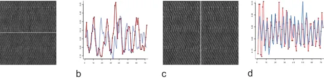
from the upper to lower part (Figure 1a-b). However, there is no significantly different of signal when we compare it from left to right one (Figure 1 c-d). The series in Figure b, lead to a conjucture that there is no defect on that line, while in Figure c, lead to a conjecture that there is defect on that line. We then test the conjecture use the proposed hypothesis test explaining in Section 2.3
Before testing those series, we first smooth the image using the 2D nonparametric approach, explaining in Section 2.1. We then use that smooth image for constructing the hypothesis test. The hypothesis test is run in each line. Suppose. we take one vector columns from Figure 1a, and let
ߤூሺݔሻǡ ݅ ൌ ͳǤ ݆ ൌ ͳǡ ǥ ǡ ݉ be the first column of the upper image, and called it series I. Let ߤூூሺݔሻǡ ݅ ൌ
ͳǤ ݆ ൌ ݉ ͳǡ ǥ ǡ ݊ be the first column of the lower image, and called it series II. We perform a test
ܪǣ ߤூ൫ݔ൯ ൌ ߤூூ൫ݔ൯ ൌ ߤ൫ݔ൯ǡ ݅ǡ ݆ ൌ ͳǡ ǥ ǡ ݊ against ܪଵǣ ߤூ൫ݔ൯ ് ߤூூ൫ݔ൯. We run the test for ݅ ൌ
ͳǡ ǥ ǡ ݊. (for simplicity, we let the image size in ݊ by ݊), and notify in which positions the test reject the
hypothesis. Those positions are regarded as the defected area in the image. Similary, the test also run from each row in Figure 1c. Running the test row-wise and columns wise then we we have a set of points which recorded the defect positions in the image. We then take the most four outer points and draw a box thougth those points for detecting the defetc area in the image.
A
b
c
d
Figure 1. The idea of comparing series from the upper to lower part and from the left to the right part
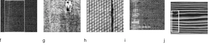
Applying the proposed methods to some defected textures, we are successfully to detect the simple defect as well as the pattern`s defect (Figure 2). Since, we take the outer points for drawing a box to detect the defect area, so in one bix box we can find several defects, i.e. Figure 2a, 2c, 2f. Therefore, we can extend the procedure for finding the defect area, so that we can find several defet areas in a image (see Figure 2d, 2i). Here, we do not use four outer points, but search points in which those points can form a box The proposed model is not running well for detecting defect for wood texture. We need to transform the image using wavelet tansformation first and then perform the test in the wavelet space, then invers the defected area in to the original space (see Figure 2j). The computation in this work was carried out using R-programming (2014).
f g h i j
Figure 2. Some examples of defect detection on pattern fabric
4. DISCUSSION AND CONCLUSION
So far, the methods presented here can handle the simple as well as the pattern defect detection in the texture. However, there are some limitations that these methods cannot overcome, and therefore should be handled in the future work. This method is not successful for capturing many defects on several locations of large texture, capturing in a complex structure such as a defect in the surface of the wood. For capturing many defects on several locations, the procedure for detecting the area of defect shold be impove, so that it can detect many areas of defects at once. So far, the four outer points defect area detection can produce too large defected area due to some small defect in the corner of the image for example. Searching some points which can detect several defect areas should be improved so that, the defected area are not too large, yet not too small to cover the defected area.
For capturing defect in a complex structure, the transformation of the image in the wavelet space is also a challenge to be considered in the future research, Since, inversing the result from the wavelet space to the original space sometime give different result as it is expected.
5. ACKNOWLEDGEMENTS
This research was supported by STEC- Sophia University, Tokyo Japan. The author has gratefully acknowledged to Prof. Akira Kawanaka, from the Sophia University Tokyo for the fruitful discussions during the author stayed in the Sophia University. The author thanks to the anonymous referee for his/her comments that improve the presentation of this paper.
6. REFERENCES
Diggle PJ, Ribeiro P. J., 2007, Model-based geostatistics. Springer, New York.
Franke, J., and Halim, S., 2007, Wild bootstrap tests: Regression models for comparing signal and images, IEEE Signal Processing Magazine, July 2007, 31-37.
Franke, J., Halim, S. and numerous co-authors, 2008, Structural adaptive smoothing procedure, in
Understanding Complex System, Springer: Heidelberg.
Fu, R., Shi, M., Wei, H., and Chen, H., 2009, Fabric defect detection based on adaptive local binary patterns, IEEE International Conference on Robotics and Biomimetics (ROBIO), 1336-1340.
Haerdle, W. and Mammen, E., 1993, Comparing nonparametric versus parametric regression fits. The Annals of Statistics, 12(4), 1926-1947.
Kumar, A., 2008, Computer-vision-based fabric defect detection a survey, IEEE Transaction on Industrial Electronics, 348-363.
Moahseri, B. B. M, Azadinia, S. and Mehbodniya, 2010, A new voting approach to texture defect detection based on multiresolutional decomposition, World Academy of Science, Engineering and Technology,65, 887-891.
Ngan, H.Y.T., Pang, G.H.K., 2009, Regularity analysis for patterned texture inspection. IEEE Trans. on Autom. Sci. and Eng.,6(1),131-144.
Ngan, H.Y.T., Pang, G.H.K., Yung, N.H.C., 2010a, Performance evaluation for motif-based patterned texture defect detection. IEEE Trans. on Autom. Sci. and Eng., 7(1), 58-72.
Ngan, H.Y.T., Pang, G.H.K., Yung, N.H.C, 2010b, Ellipsoidal decision regions for motif-based patterned fabric defect detection. Pattern Recognition, 43, 2132-2144
R-programming, 2014, www.r-project. org.
Tang, L., Schucany, W. R., Woodward, W. A., and Gunst, R. F., A spatial bootstrap, Technical Report, Department of Statistical Science, University of Southern Methodist, [Online] Available: http://smu.edu/statistics/techreports/tr337.pdf (retrieved in June 2011)