Full Terms & Conditions of access and use can be found at
http://www.tandfonline.com/action/journalInformation?journalCode=cbie20
Download by: [Universitas Maritim Raja Ali Haji] Date: 19 January 2016, At: 20:21
Bulletin of Indonesian Economic Studies
ISSN: 0007-4918 (Print) 1472-7234 (Online) Journal homepage: http://www.tandfonline.com/loi/cbie20
Revisiting growth and poverty reduction in
Indonesia: what do subnational data show?
Arsenio M. Balisacan , Ernesto M. Pernia & Abuzar Asra
To cite this article: Arsenio M. Balisacan , Ernesto M. Pernia & Abuzar Asra (2003) Revisiting growth and poverty reduction in Indonesia: what do subnational data show?, Bulletin of Indonesian Economic Studies, 39:3, 329-351, DOI: 10.1080/0007491032000142782 To link to this article: http://dx.doi.org/10.1080/0007491032000142782
Published online: 03 Jun 2010.
Submit your article to this journal
Article views: 341
View related articles
INTRODUCTION
By international standards, Indonesia has done remarkably well in the areas of both economic growth and poverty reduction. For two decades before the Asian financial crisis in the late 1990s, economic growth averaged 7% p.a. This was the norm for East Asia, and was substantially higher than the aver-age growth rate of 3.7% for all devel-oping countries. At the same time, Indonesia’s poverty incidence fell from 28% in the mid 1980s to about 8% in the mid 1990s, compared with a decline for all developing countries (excluding China) from 29% to 27%.1
Indonesia’s record also compares well with those of China and Thailand, whose economies grew at an even faster rate.
The Asian financial crisis, exacer-bated by domestic political turbulence, hit the Indonesian economy hard. GDP per capita contracted by 13% in 1998, effectively returning it to its 1994 level. Poverty rose sharply, as indicated by both official and independent esti-mates.2Official figures issued by Indo-nesia’s Central Statistics Agency (BPS, Badan Pusat Statistik) show the pro-portion of people deemed poor
increas-REVISITING GROWTH AND POVERTY
REDUCTION IN INDONESIA:
WHAT DO SUBNATIONAL DATA SHOW?
Arsenio M. Balisacan
University of the Philippines-Diliman and SEAMEO Regional Center for Graduate Study and Research in Agriculture
Ernesto M. Pernia
Asian Development Bank, Manila
Abuzar Asra*
Asian Development Bank, Manila
Indonesia has an impressive record of economic growth and poverty reduction over the past two decades. The growth–poverty nexus appears strong at the aggre-gate level. However, newly constructed panel data on the country’s 285 districts reveal huge differences in poverty change, subnational economic growth and local attributes across the country. The results of econometric analysis show that growth is not the only factor to affect the rate of poverty change; other factors also directly influence the welfare of the poor, as well as having an indirect effect through their impact on growth itself. Among the critical ones are infrastructure, human capital, agricultural price incentives and access to technology. While fostering economic growth is crucial, a more complete poverty reduction strategy should take these relevant factors into account. In the context of decentralisation, subnational analy-sis can be an instructive approach to examining local governance in relation to growth and poverty reduction.
ISSN 0007-4918 print/ISSN 1472-7234 online/03/030329-23 © 2003 Indonesia Project ANU DOI: 10.1080/0007491032000142782
ing from 17.7% in 1996 to 24.2% in 1998. But just as the economic contraction caused a sharp increase in the poverty rate, the rebound in 1999 and 2000, albeit modest, caused it to fall, nearly to its pre-crisis level. Based on independ-ent estimates (Suryahadi et al. 2000), poverty incidence in late 1999 had fallen to 10%, comparable to the level in early 1996, after shooting up to 16% in mid 1998. These estimates suggest that poverty in Indonesia responds rela-tively strongly and quickly to large shocks.
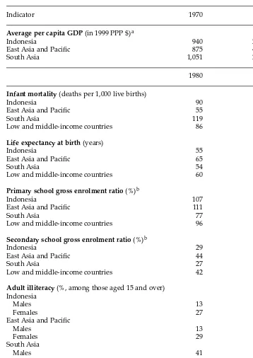
While the Asian crisis adversely affected the welfare of the Indonesian people, the country’s achievements in economic and human development over the past quarter-century remain impressive, especially when viewed against the performance of South Asia and other low and middle-income countries (table 1). The economic and social gains from the high-growth period could not be wiped out so easily.
Indonesia’s overall growth and poverty reduction experience appears to approximate the findings of studies based on cross-country regressions. Dollar and Kraay (2001), for example, show that the incomes of the poor move one for one with overall average incomes, suggesting that poverty reduction requires nothing much more than to promote rapid economic growth.
There is more to the growth–poverty nexus, however, than the national averages would imply. Growth and poverty reduction vary enormously across the island groups, provinces and kota/kabupaten (urban and rural districts) of Indonesia.3In recent years, this variance appears to be widening rather than converging; and given its ethnic dimensions, this is becoming a politically sensitive issue (Hill 2002). Recent history is replete with examples
to show that social or political tensions arising from economic disparities tend to dampen the return to high growth, thus making it more difficult to win the war against poverty.
An appropriate approach to socio-economic disparities requires a clear understanding of the policy and insti-tutional factors that account for differ-ences in the evolution of growth and poverty in the various districts of Indonesia. To what extent can differ-ences in growth explain the observed differences in poverty reduction across provinces and districts? How impor-tant are government policies and pro-grams, as well as geographic attributes and local institutions, in influencing poverty? What lessons can be learned from recent experience to promote poverty reduction in the poorest areas? As a case study for addressing the above questions, Indonesia offers advantages not found in many other developing countries. First, as already noted, the country is diverse both in its geographic and institutional attributes and in the economic performance of its provinces and districts. It is this diver-sity that permits an assessment of the influence of economy-wide policies and ‘initial’ conditions of poverty. And second, comparable cross-sectional and time-series data on subnational units of government (provinces and districts) are available for the 1990s, a period characterised by marked changes in the policy environment and economic performance. This facilitates a sufficiently disaggregated analysis to enhance our understanding of the determinants of growth and poverty reduction.
This paper examines the key deter-minants of poverty reduction in Indonesia during the 1990s. The fol-lowing section describes data and measurement issues. The third section
TABLE 1 Selected Social Indicators: Indonesia versus Other Developing Countries
Indicator 1970 2000
Average per capita GDP (in 1999 PPP $)a
Indonesia 940 2,882
East Asia and Pacific 875 4,413
South Asia 1,051 2,216
1980 1999
Infant mortality (deaths per 1,000 live births)
Indonesia 90 42
East Asia and Pacific 55 35
South Asia 119 74
Low and middle-income countries 86 59
Life expectancy at birth (years)
Indonesia 55 66
East Asia and Pacific 65 69
South Asia 54 63
Low and middle-income countries 60 64
Primary school gross enrolment ratio (%)b
Indonesia 107 113
East Asia and Pacific 111 119
South Asia 77 100
Low and middle-income countries 96 107
Secondary school gross enrolment ratio (%)b
Indonesia 29 56
East Asia and Pacific 44 69
South Asia 27 49
Low and middle-income countries 42 59
Adult illiteracy (%, among those aged 15 and over) Indonesia
Males 13 9
Females 27 19
East Asia and Pacific
Males 13 8
Females 29 22
South Asia
Males 41 34
Females 66 58
Low and middle-income countries
Males 22 18
Females 39 32
aPPP: purchasing power parity. Figures are three-year averages, centred on the year shown. bThe most recent data on primary and secondary school enrolments are for 1997.
Sources: World Bank (2001); IMF (2001).
uses consistently assembled district-level data to analyse the basic growth– poverty relationship. The fourth sec-tion probes the contribusec-tion of local attributes and time-varying economic factors to the variation in district-level economic performance vis-à-vis
changes in poverty. A main interest here is in assessing the extent to which certain policy measures can enhance or diminish the impact of growth on the living standards of the poor. The paper concludes by assessing implications for the design of pro-poor, growth-oriented policies and institutions in Indonesia.
DATA AND MEASUREMENT ISSUES
The National Socio-economic Survey (Susenas, Survei Sosial Ekonomi Nasional) conducted by the BPS is the main source of data for analyses of poverty and inequality. The survey comes in two sets: the consumption module and the core data, hereafter referred to as the Susenas module and the Susenas core. The Susenas module provides detailed consumption data, is undertaken every three years, and allows disaggregation only at the provincial level. For the 1990s, such data are available for 1993, 1996 and 1999. The Susenas core, on the other hand, covers both consumption and other socio-economic indicators on an annual basis, with the specific indica-tors varying from year to year. The consumption data in the Susenas core are not as detailed as those in the Suse-nas module and, indeed, give a differ-ent picture of the level of consumption: the consumption figures for 1993–99 from the Susenas core are about 11% lower, on average, than those from the Susenas module. The advantage of the Susenas core is that the data allow
dis-aggregation at the district level. Offi-cial government poverty figures calcu-lated by the BPS are based on the Suse-nas module.4
We use the Susenas core, as its cov-erage of 285 districts—versus 26 provinces for the Susenas module— yields a far greater number of observa-tions for each survey year.5However, to obtain the same aggregate poverty profile as that given by the Susenas module, we have adjusted the con-sumption data from the Susenas core such that the consumption expendi-ture means by quintile correspond to those obtained from the Susenas module.
On both conceptual and practical grounds, consumption is preferable to income as a measure of household wel-fare. Microeconomic theory suggests that since welfare level is determined by ‘life-cycle’ or ‘permanent’ income, and since current consumption is a good approximation of this income, current consumption is an appropriate measure of both present and long-term well-being. Indeed, measured con-sumption is typically less variable than measured income (Deaton 2001). For practical purposes, it is less difficult to acquire accurate information on con-sumption than on income, especially in developing countries where the gover-nance infrastructure is weak and local markets are relatively undeveloped (Deaton 1997; Ravallion and Chen 1997; Srinavasan 2001).
The National Income Accounts (NIA) are another distinct source of data on average welfare. Although GDP per capita is widely used to meas-ure welfare, the level of personal con-sumption expenditure (PCE) per capita is closer to the concept of average wel-fare, as measured by households’ com-mand over resources. In general, PCE as measured in the NIA, and
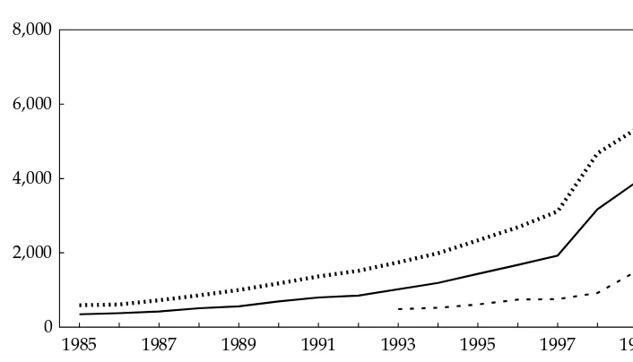
hold consumption expenditure (HCE) as measured in the Susenas, do not necessarily correspond either as to level or growth rate, largely because of differences in definitions, methods and coverage.6 For example, PCE may exceed HCE simply because it lumps together spending by the non-profit sector (non-government organisations, religious groups, political parties) with spending by the household sector. At any rate, in the Indonesian case, aver-age per capita levels of PCE and HCE move broadly in the same direction, at least for the 1990s (figure 1).
The chosen indicator of household welfare, per capita consumption expen-diture, has to be adjusted for spatial cost-of-living, or SCOL, differences because prices in any given year vary substantially across provinces and dis-tricts. The SCOL index is simply the ratio of the cost of attaining a level of
utility in province k to the cost of attaining it in a reference province, r. To the extent that spatial poverty lines are comparable in utility terms (that is, imply the same standard of living), then the ratio of the poverty line for province k to that of the reference province r is an appropriate SCOL index. For our purposes, we use the 1999 official poverty lines for urban areas to approximate SCOL differences among the 26 provinces, as periodic surveys to construct the consumer price index (CPI) cover only urban areas. Using urban poverty lines and Jakarta as the reference province (Jakarta = 100), we find large inter-provincial differences in the cost of liv-ing, ranging from 74% in Southeast Sulawesi to 116% in Bengkulu (appen-dix table 1).
Comparison of household welfare over time requires that the chosen
FIGURE 1 Average per Capita Expenditure: National Income Accounts versus Susenas (Rp ’000 at current prices)
1985 1987 1989 1991 1993 1995 1997 1999
0 2,000 4,000 6,000 8,000
GDP per capita PCE per capita HCE per capita
PCE: personal consumption expenditure; HCE: household consumption expenditure.
Sources: National Income Accounts; Susenas.
welfare indicator, consumption expen-diture, be adjusted for nominal price movements during the 1990s. A straightforward way to achieve this would be to deflate the SCOL-adjusted consumption expenditures using province-specific CPIs.7 For practical purposes, this would be sufficient if price movements had been uniform across consumer goods during the period of interest. However, in reality price movements varied across con-sumption items, especially during the economic crisis of the late 1990s.
We have constructed a CPI for each income quintile of the population to take account of the differential price regimes faced by each group. The con-struction involves combining the infor-mation on province-specific CPIs with the district-level expenditure shares (weights), based on the 1996 Susenas core, of each population quintile in the following commodity groups: food; prepared food and beverages; housing; clothing; health, education and recre-ation; and transport and communica-tion. Table 2 summarises the results for 1993–99.
Because of the sharp rupiah
depreci-ation from July 1997, overall price inflation was much higher in 1996–99 (at 121%) than in 1993–96 (27%). In addition, while price changes did not vary much across quintiles between 1993 and 1996 (the pre-crisis period), they did vary greatly between 1996 and 1999 (the crisis period). During the latter period, consumer price inflation was about 128% for the bottom quin-tile, compared with only 109% for the top quintile. The very high inflation rate for the poor during the crisis period was caused by marked increases in the prices of food, particu-larly rice, which accounts for a domi-nant share of the poor’s consumption basket (Sigit and Surbakti 1999).8
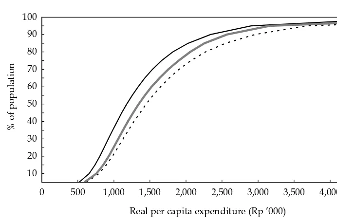
The resulting national distribution of per capita consumption expendi-tures for the three Susenas years is shown in figure 2. Note that the expen-ditures are in real terms (at 1999 prices) and have been adjusted for provincial cost-of-living differences. Thus, with the poverty line (in real terms) known, it is straightforward to obtain poverty incidence for the various years from figure 2. For example, if the national average (population-weighted) official
TABLE 2 Consumer Price Index by Expenditure Quintile
1993 1996 1999 % Change
1993–96 1996–99
National average 100.0 127.3 281.3 27.3 121.0
Quintile
First (poorest) 100.0 128.2 292.2 28.2 128.0
Second 100.0 127.9 288.4 27.9 125.6
Third 100.0 127.6 284.6 27.6 123.1
Fourth 100.0 127.2 279.1 27.2 119.5
Fifth (richest) 100.0 126.1 264.0 26.1 109.4
Source: Susenas.
poverty line of about Rp 904,400 per person is used, the resulting poverty incidence would be 26% for 1993, 13% for 1996 and 16% for 1999.9
As shown by Foster and Shorrocks (1988), two non-intersecting cumula-tive distribution curves will suggest that the direction of poverty change is unambiguous even for all other plausi-ble poverty indices that satisfy certain properties of a desirable poverty meas-ure. As figure 2 shows, this is the case for 1993 and 1996, as well as for 1996 and 1999. Thus, poverty is unambigu-ously higher in 1999 than in 1996, but still much lower than in 1993, for virtu-ally all poverty norms and standard poverty measures that have been sug-gested in the literature.
To some extent, the pattern of poverty change shown above is quali-tatively consistent with the observa-tions reported in previous studies. Using their ‘consistent’ estimates,
Sury-ahadi et al. (2000) found that poverty increased by 6.5 percentage points between 1996 and 1999; based on offi-cial poverty lines, the ADB (2000) found that it rose by roughly six percentage points. We estimate that the poverty rate increased by approxi-mately three percentage points between 1996 and 1999. Note, however, that this takes account of substantial inter-provincial differences in the cost of living.
A caveat on the welfare distribution estimates for 1996 and 1999 is in order. The difference between the two years is strictly not an estimate of the extent of change during the crisis. The crisis did not begin in February 1996 and end in February 1999, the months in which the Susenas data used in this paper were collected. Economic growth continued to be positive and to surpass popula-tion growth (while inflapopula-tion remained moderate) for nearly a year and a half
Source:Susenas.
FIGURE 2 Distribution of Per Capita Consumption
10 20 30 40 50 60 70 80 90 100
0 500 1,000 1,500 2,000 2,500 3,000 3,500 4,000 4,500
% of population
Real per capita expenditure (Rp ’000)
1993 1996 1999
after the 1996 survey. This could have caused a further decline in poverty, in line with the norm for the 1980s and the first half of the 1990s. Thus, the increase in poverty during the crisis was proba-bly higher than the three percentage points shown in figure 2.
SUBNATIONAL DIFFERENCES IN WELFARE
The available data show large differ-ences in natural endowment, agrarian
structure, institutions, policies and access to support services across the country’s 285 districts. Figure 3 high-lights these differences for a few indi-cators, namely schooling, farm charac-teristics and access to infrastructure, technology and finance. These indica-tors (some of which are discussed in more detail in the next section) are district-level averages for the 1990s. In general, the values for districts are scattered widely around the overall (national) mean for each indicator. The
Log (mean expenditure)
Log (mean expenditure)
FIGURE 3 District-level Differences for Selected Indicators (indices)
Schools: District average for the distance of villages from the nearest junior secondary school and the nearest senior secondary school.
Information: District average for the proportion of villages with: public phones; public televi-sion; and post offices.
Electricity: Proportion of villages in district with state-run electricity. Roads: Proportion of villages in district with paved roads.
dispersion is quite substantial even for districts with similar levels of real per capita expenditure.
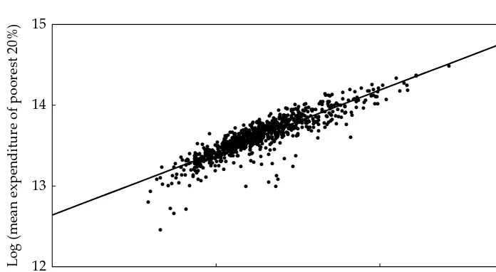
District-level data covering the three survey years (a total of 855 observa-tions) reveal a strong positive correla-tion between district-level average expenditure and the average expendi-ture of the poorest 20% of the popula-tion (figure 4).10 The relationship is
summarised by the fitted line, which is obtained by ordinary least squares (OLS) regression of the mean welfare of the poor on overall mean expendi-ture (income).11 Note that both means are expressed in logarithms; hence the slope of the fitted line can be inter-preted as the elasticity of the average income of the poor with respect to overall mean income, henceforth
Agricultural workers
Log (mean expenditure)
Farm size
Log (mean expenditure)
FIGURE 3 (continued) District-level Differences for Selected Indicators (indices)
Finance: District average for the proportion of villages with a bank and the proportion with a cooperative.
Farm size: Average farm size (ha).
Irrigation: Ratio of total irrigated area to the total area comprising wetlands, garden drylands, shifting cultivation lands and grasslands.
Agricultural worker households: Ratio of agricultural labourer households to total agricultural households.
Sources: BPS, Village Potential Statistics (Podes) for 1993, 1996 and 1999; BPS, Jakarta.
referred to as the growth elasticity of poverty. This elasticity is about 0.8, indicating that a 10% increase in district-level income raises the living standards of the poor by 8%.12 This result is strikingly similar to Bhalla’s (2001) estimate, based on cross-country analysis, of poverty reduction from the late 1980s to the late 1990s.
However, simply regressing the per capita income of the poor on overall per capita income is likely to yield an inconsistent estimate of the growth elasticity of poverty. Measurement errors in per capita income (which is also used to construct our measure of the average income of the poor) bias the estimate of this elasticity. More-over, it is possible that the incomes of the poor and overall incomes are jointly determined. Recent theory and evidence show a link between inequal-ity (hence, the incomes of the poor) and subsequent overall income growth. One school of thought sug-gests that income (or asset) inequality inhibits subsequent overall income growth (Alesina 1998; Deininger and Squire 1998); another posits the reverse
(Forbes 2000; Li and Zou 1998). Incon-sistency in the parameter estimates of the growth–poverty relationship in fig-ure 4 may also arise from the omission of variables that have a direct impact on the welfare of the poor and are cor-related with overall average income (figure 3). Provincial indicators of human capital, infrastructure and local institutions (for example, social capi-tal) appear to be strongly correlated with provincial mean incomes (Booth 2000; Kwon 2000: Garcia Garcia 1998). We address these statistical prob-lems by checking the robustness of the growth elasticity estimates and explor-ing other determinants of district-level poverty reduction. Figure 5 sum-marises our empirical approach.
To deal with the measurement error, we could use average income to instru-ment for average expenditure. How-ever, the income variable is not avail-able at the district level. The alternative instrument is district-level expenditure growth, which also takes care of the endogeneity issue.13In the case of the omitted-variables bias problem, we exploit the longitudinal nature of the
FIGURE 4 Welfare of the Poor versus District Mean Expenditure
Log (mean expenditure of poorest 20%)
Log (district-level mean expenditure)
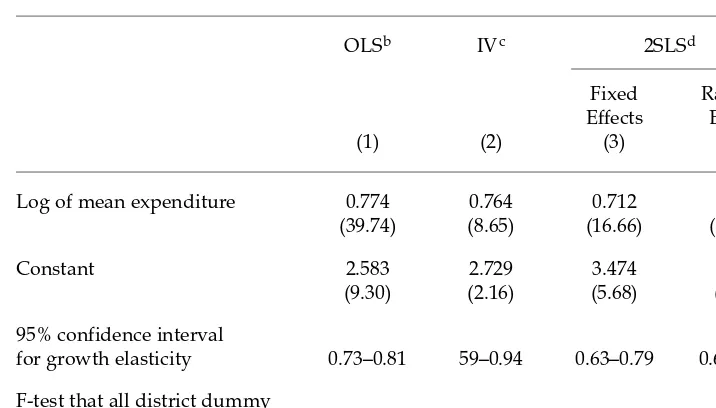
district-level data and employ panel estimation techniques to control for differences in time-invariant, unob-servable district-specific characteris-tics. Specifically, we use two standard panel estimation models—the fixed effects model and the random effects model—suited to addressing un-observed fixed-effects problems, but in such a way that the endogeneity of overall mean income is observed.14 Table 3 summarises the results of the estimation. For comparison, we also show the OLS regression estimates implied by the fitted line in figure 4, as well as the instrumental variable (IV) regression estimates.
The panel estimation results indi-cate that the unobserved district-specific effects are indeed significant, leading to a reduction in the earlier OLS estimate of the growth elasticity of poverty (of nearly 0.8) to about 0.7. Both panel estimation techniques give roughly the same elasticity estimate, including the values at the 95% confi-dence interval. Hence, we employ the
panel estimation technique, in particu-lar the fixed effects model, which also allows for the endogeneity of the over-all income variable. The assumption of the random effects model that the unobserved district-level effects and the explanatory variables are uncorre-lated is not supported by the data. This correlation problem also applies to the IV estimation technique.
To sum up, our estimate of the growth elasticity of poverty is not nearly the one-for-one correspondence between increase in the welfare of the poor and growth in overall income found in studies employing cross-country regressions. However, the esti-mate for Indonesia is higher than that for the Philippines; a similar study for the latter country found this elasticity to be about 0.5 (Balisacan and Pernia 2002). The comparison is instructive since the two countries are at roughly similar stages of economic develop-ment. Thus, while other factors appear to have direct (distributive) effects on the welfare of the poor, in the
Indone-FIGURE 5 Empirical Frameworka
aReverse causation running from welfare of the poor (average per capita expenditure) to
growth (overall average per capita income) is not shown.
Welfare of the poor
Per capita expenditure
Overall average per capita
income
Policy regime Political attributes Infrastructure Geographic attributes Technology Agricultural land Finance attributes
Growth Other factors
sian case changes in the welfare of the poor in response to overall economic growth seem fairly large. This could be explained by the relatively more labour-intensive and agriculture-based nature of economic growth in Indone-sia. Over the past two decades, the rate of agricultural sector growth has been significantly higher in Indonesia than in the Philippines: 3.7% in the 1980s and 2.2% in the 1990s for Indonesia compared with 1.9% and 1.8% for the Philippines.
OTHER FACTORS INFLUENCING POVERTY REDUCTION
Certain economic and social factors influence poverty reduction at the local level. These include overall per capita
income, relative price incentives, human capital and access to infra-structure, technology and finance. We use these variables to explain the wide differences in the per capita incomes of the poor across Indonesia’s 285 dis-tricts during the 1990s. Guiding our specifications are development theory, data availability, and estimation sim-plicity.
The proxy for the human capital variable is the district-level average years of schooling of household heads. This is expected to influence the wel-fare of the poor directly (through income distribution), apart from its effect on district-level income growth. Numerous studies suggest that the higher the level of educational attain-ment, the higher a person’s expected
TABLE 3 Basic Specifications: Elasticity of the Income of the Poor to Overall Incomea
OLSb IVc 2SLSd
Fixed Random Effects Effects
(1) (2) (3) (4)
Log of mean expenditure 0.774 0.764 0.712 0.714 (39.74) (8.65) (16.66) (20.95)
Constant 2.583 2.729 3.474 3.442
(9.30) (2.16) (5.68) (7.05)
95% confidence interval
for growth elasticity 0.73–0.81 59–0.94 0.63–0.79 0.65–0.78
F-test that all district dummy
coefficients are zero 5.58
aThe dependent variable is the logarithm of the mean expenditure of the bottom 20% of
the population. Except for OLS, all estimations instrument for mean expenditure using lagged mean expenditure growth. Figures in parentheses are t-ratios. Data refer to a panel of 285 districts surveyed in 1993, 1996 and 1999.
bOLS: ordinary least squares.
cIV: instrumental variable.
d2SLS: two-stage least squares.
earnings over a lifetime (see, for exam-ple, Krueger and Lindhal 2001). For urban Java, the private rate of return to education is about 17%, higher than in most other countries (Byron and Taka-hashi 1989, cited in Lanjouw et al.2001). The social rate of return is also quite high, at roughly 14% for junior second-ary education and 11% for senior sec-ondary education (McMahon and Boe-diono 1992).
Two alternative proxies for human capital are adult literacy and access to basic schooling. The first is defined as the proportion of the adult population who can read and write. The second is the average distance of a district’s vil-lages from a secondary (junior and senior high) school. As is well known, since the late 1960s Indonesia has wit-nessed an enormous expansion of edu-cational opportunities at all levels. Duflo (2001) found that each primary school constructed per 1,000 children led to an average increase of 0.12–0.19 years of education, as well as a 1.5–2.7% increase in wages. Household data suggest, however, that whereas univer-sal primary enrolment was reached as early as around 1986, the level of sec-ondary enrolment still varied enor-mously across provinces in the 1990s (Lanjouw et al.2001; see also figure 3). This large degree of variation was true not only between islands, or between Java and the rest of the country, but also between provinces on the major islands. For example, while West Kali-mantan did poorly in terms of educa-tion and poverty outcomes, the situa-tion was far less worrisome in Central Kalimantan.
Roads represent the infrastructure required to access markets, off-farm employment and social services. This variable, defined as the proportion of villages with paved roads, may be seen as an indicator of spatial connectivity
or, conversely, of spatial isolation implying geographic ‘poverty traps’.15 The presence of natural resources (oil, gas and minerals) is expected to influence growth and poverty reduc-tion. This is defined in terms of the rel-ative importance of oil and gas in the local economy. The net effect of this variable on the welfare of the poor in resource-rich areas is, however, not a priori obvious.
The price incentives variable is given by the local terms of trade, defined as the ratio of agricultural product prices to non-agricultural product prices. Since poverty is con-centrated in agriculture in developing countries (Pernia and Quibria 1999), including Indonesia (Asra 2000), this variable is expected to have a positive influence on the incomes of the poor.
Electricity is a proxy for access to technology, or simply the ability to use modern equipment. It is defined as the proportion of villages with access to state-run electricity. The communica-tion–information variable also serves as an indicator of access to technology. It is given here by a composite index representing the proportion of villages with access to public telephones, tele-vision, post offices and newsagents (appendix table 2). We further combine the electricity and communication– information variables into a single composite index referred to simply as ‘technology’. This variable is expected to positively influence the welfare of the poor, apart from its positive impact on overall growth.
Access to credit is critical to manag-ing household consumption, particu-larly as far as the poor are concerned, because it affords them the means to smooth their incomes in the event of unfavourable shocks. It is likewise crit-ical in securing working capital, main-taining assets and expanding
342
Arsenio M. Balisacan, Ernesto M. Pernia and
Abuzar
Asra
TABLE 4 Determinants of the Welfare of the Poora
(1) (2) (3) (1a) Explanatory Regression FSFE Regression FSFE Regression FSFE Regression FSFE Variable Estimate Estimate Estimate Estimate
(mean years of schooling of first quintile) Overall mean income (Y) 0.7244*** 0.7144*** 0.7149*** 0.7228***
(13.12) (13.42) (13.42) (13.76) Human capital
Years of schooling –0.0392 0.0447 0.0166** –0.0034 (–0.40) (0.60) (1.88) (–0.51) Adult literacy 0.1290 0.3107**
(0.74) (2.32)
Distance to schools –0.0173 0.0166 (–1.19) (1.50)
Terms of trade 0.0006* 0.0014*** 0.0005 0.0013** 0.0006* 0.0014*** 0.0006* 0.0014*** (1.77) (4.83) (1.35) (4.57) (1.64) (5.04) (1.63) (4.94) Technology 0.2153* 0.0287 0.2063* 0.0436 0.2046* 0.0402 0.2266** 0.0319 (1.84) (0.33) (1.77) (0.50) (1.76) (0.46) (1.97) (0.35) Finance 0.0351 –0.0058 0.0428 –0.0124 0.0335 –0.0044
(0.48) (–0.10) (0.58) (–0.22) (0.45) (–0.08)
Roads –0.0143 0.0499** –0.165 0.0320 –0.0116 0.0479** –0.0176 0.0516*** (–0.52) (2.34) (–0.56) (1.41) (–0.42) (2.26) (–0.79) (2.53) Oil and gas –0.1927 0.3843** –0.2948 0.3641** –0.2284 0.4253*** –0.2691 0.4155***
(–0.90) (2.35) (–1.36) (2.21) (–1.09) (2.64) (–1.28) (2.56) Lagged growth of Y 0.4566*** 0.4678*** 0.4611*** 0.4583***
(24.18) (24.8) (24.76) (24.95) Intercept 3.2778* 13.9773*** 3.2659*** 13.8259*** 3.2958* 14.1001*** 3.1629*** 14.0700***
(4.23) (101.54) 4.14 (131.32) 4.27 (277.83) (4.15) (280.79)
R-squared 0.741 0.785 0.739 0.789 0.732 0.787 0.733 0.785
F-ratio 145.11 145.23 146.37 169.81 Wald X2(×1,000) 24,141 23,759 24,267 24,507
Prob > X2 0 0 0 0
F-test that all fixed effects are zero 4.49 4.69 4.67 3.46 No. of observations 570 558 570 570
nesses. This variable is defined as the district average for the proportion of villages with a bank and the propor-tion with a cooperative.
Table 4 summarises the results of the econometric estimation, including the results of the first-stage fixed effects regression (FSFE), which indicate the response of overall growth to the exogenous variables. Appendix table 2 provides the descriptive statistics on the variables.
After controlling for the influence of other factors (including unobserved district-specific fixed effects), the growth of overall income appears to exert a significant influence on the incomes of the poor. Indeed, the esti-mate of the growth elasticity is quite robust, consistently around 0.7 in the various specifications. Surprisingly, this estimate is close to that obtained in the basic specifications in which district-specific effects are controlled for (regressions 3 and 4 in table 3).
Evidence on the direct effect of schooling is mixed. The variable for mean years of schooling is insignificant (regression 1), as is the variable for dis-tance to school (regression 3). Note, however, that the variable for mean years of schooling is significant if it is defined for the poor only (regression 1a). It is possible that years of schooling may not adequately reflect differences in human capital across the income spectrum. However, for the poor, the number of years at school may corre-spond closely to achieved human capi-tal since school quality may be less heterogeneous within the group.
Adult literacy also appears not to have a direct impact on the welfare of the poor (regression 2). However, it exerts a significant influence on overall growth, suggesting that an improve-ment in human capital reduces poverty principally through the growth
pro-cess. In other words, investment in human capital promotes growth, there-by indirectly reducing poverty.
Price incentives matter to poverty reduction, as indicated by the positive and significant coefficient of the terms of trade variable. This means that changes in the price of agriculture rela-tive to the price prevailing in other sec-tors of the local economy have an impact on the welfare of the poor, both directly by affecting income redistribu-tion and indirectly through their posi-tive effect on overall growth.16 It is worth noting that the country’s price and trade policy regimes in the 1980s and 1990s tended to penalise agri-culture relative to manufacturing. Although significant trade reforms took effect in the 1980s and 1990s, directly conferring some protection on the primary sector, the protection regime as a whole has continued to tax agriculture, though to a lesser extent (Garcia Garcia 2000). This would have limited the income gains from trade reform in provinces dependent on agriculture. Evidently, since agricul-ture is more tradable than either indus-try or services, and since agriculture is more labour-intensive than industry, reducing trade and price distortions promotes both poverty reduction and growth objectives.17
The technology variable is positive and significant, supporting the expec-tation that it matters to the incomes of the poor. Recall that this refers to the availability of electricity and publicly provided information channels at the village level. Villagers in areas where these services are absent may simply not have an important avenue for rais-ing the productivity of their assets (in agriculture, mainly land and labour). The coefficient estimates, which aver-age around 0.2, suggest that a 10% improvement in access to these
ices raises the incomes of the poor by roughly 2%, other things being equal.
Surprisingly, the finance variable is insignificant. This runs counter to the common claim that access to formal financial intermediaries, particularly in agriculture, is critical for poor peo-ple. It may be that this variable is a poor proxy for access to credit.18 The specific location and scale of financial intermediaries vis-à-visthe village pop-ulation might be a better indicator, but data on such a variable are not avail-able. Moreover, the proxy finance vari-able correlates strongly with the tech-nology variable. Nevertheless, deleting the finance variable in the estimating model does not significantly change the parameter estimates of the remain-ing variables.
The roads variable does not appear to be significant, but it has a strong impact on overall growth. This is con-sistent with the observation by, for example, Hill (1996) that the public provision of roads is designed not as a vehicle for achieving intradistrict (or intraprovince) redistribution, but rather as part of a development strat-egy to spur economic growth, espe-cially in the countryside.
The variable representing natural resources is not significant, although it does significantly influence overall growth. This supports the observation by Tadjoeddin, Suharyo and Mishra (2001) that there is no strong correla-tion between natural resource endow-ment and community welfare, defined in terms of human development indi-cators (HDI).19The revenues generated by natural resources have, however, been an important means of financing development projects, especially those aimed at keeping interregional inequal-ity low. Indeed, the New Order gov-ernment’s equalisation policy—which was achieved mainly through fiscal
policy instruments such as central gov-ernment transfers, interregional trans-fers and other initiatives within the Special Presidential Program (Inpres) for poor villages—was quite effective in spurring growth outside the Java– Bali enclave, especially in the Outer Island provinces.
DIFFERENTIAL EFFECTS ACROSS QUINTILES
Do the welfare effects of the economic and social factors discussed in the pre-ceding section vary across income groups? The growth elasticity esti-mates of less than unity shown in tables 3 and 4 indicate that people in the upper ranges of the income distri-bution tend to benefit more than pro-portionately from overall economic growth. What policies or institutional arrangements might enhance the bene-fits of growth for the poor?
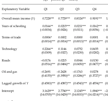
We estimate the model for each of the other four income quintiles. In par-ticular, we focus on the variant of the model in which the finance variable is dropped and the schooling variable pertains to the mean years of schooling for the relevant quintile.20 Recall that in the earlier variant we used the mean schooling years of the first quintile, rather than the overall mean schooling years of all quintiles, as a regressor. This education variable yielded a posi-tive and significant impact on the wel-fare of the poor. The estimation results for each quintile are summarised in table 5. For ready comparison, the results reported in table 4 for the first quintile (column 1a) are reproduced as the first column in table 5.
Results for the other quintiles gener-ally do not diverge greatly from those for the first quintile. Apart from district mean income, average schooling in each income group directly and
tively influences the welfare of that group, as expected. Natural resource endowment (oil and gas), infrastruc-ture (roads) and terms of trade exert an influence on welfare through their pos-itive impact on overall income growth.
The growth elasticity of welfare tends to increase monotonically with the income quintile, suggesting that
people in the higher income groups do indeed enjoy more of the benefits of growth. Similar results have been found for the Philippines, except that the growth elasticities for the first two quintiles (the bottom 40% of the popu-lation) are significantly lower.
It is also worth noting that the returns to schooling are fairly similar
TABLE 5 Determinants of Average Welfare by Quintilea (Q1 = poorest; Q5 = richest)
Explanatory Variable Q1 Q2 Q3 Q4 Q5
Overall mean income (Y) 0.7228*** 0.7729*** 0.8324*** 0.9191*** 1.1900***
Years of schooling 0.0166** 0.0215*** 0.0211*** 0.0162*** 0.0164*** (–0.0034) (0.0026) (0.0111) (0.0056) (–0.0043)
Terms of trade 0.0006* 0.0002 0.0000 0.0001 0.0001 (0.0014)*** (0.0014)*** (0.0013)*** (0.0014)*** (0.0014)***
Technology 0.2266** 0.1146 0.0752 0.0655 0.1626** (0.0309) (0.0327) (0.0230) (0.0282) (0.0412)
Roads –0.0176 0.0215 0.0044 0.0150 –0.0199
(0.0516)*** (0.0484)** (0.0450)** (0.0477)** (0.0496)**
Oil and gas –0.2691 –0.2628 –0.1763 0.0278 0.0280 (0.4155)*** (0.3950)** (0.3286)** (0.3727)** (0.4086)***
Lagged growth of Y (0.4583)*** (0.4587)*** (0.4543)*** (0.4554)*** (0.4645)***
Intercept 3.1629*** 2.7740*** 2.1245*** 1.0940*** –2.2130*** (14.0705)*** (14.0429)*** (14.0033)*** (14.0214)*** (14.0910)***
Wald X2(×1,000) 24,504 54,710 70,432 94,042 52,379
Prob > X2 0 0 0 0 0
*** denotes significance at the 1% level; ** denotes significance at the 5% level; * denotes significance at the 10% level.
aEstimation is by two-stage least squares (2SLS) fixed effects regression. The dependent
variable is the logarithm of the quintile mean per capita expenditure adjusted for provin-cial cost-of-living differences. Figures in parentheses are the results of first-stage fixed effects (FSFE) regressions in which the dependent variable is the logarithm of the district mean per capita expenditure.
across quintiles. An additional year of schooling raises per capita income by roughly 2%, other things being equal.21 This result thus affirms the common claim in the development literature that education represents an important avenue for raising household wel-fare—even more so for the poor, whose access to land and other assets is very limited. Finally, it appears that access to technology directly influences the welfare of the poorest and the richest quintiles, but not those in between.
CONCLUSION
Newly constructed panel data on Indonesia’s 285 districts reveal huge differences in poverty change, sub-national economic growth and local attributes across the country. Econo-metric analysis of these data shows that the welfare of the poor responds quite strongly to overall income growth: the growth elasticity of poverty is about 0.7. This growth–poverty nexus seems significantly stronger than in the Philippines, where the elas-ticity is estimated to be only about 0.5. This may be explained by the higher growth rate of agriculture in Indone-sia, which is likely to have been more employment generating. Still, the growth–poverty relationship is far from the one-to-one correspondence revealed by studies based on cross-country regressions. Growth is good for the poor in Indonesia, as in the Philippines, but it is not good enough. Factors other than economic growth exert direct distributive effects on the welfare of the poor, apart from their impact on growth itself. Among the critical ones are the terms of trade regime, schooling, infrastructure and access to technology. Although often referred to in the literature as being important to the poor, the access to
credit variable as defined by available data was not significant. Future work must go beyond physical indicators of financial services to include ‘meso’ indicators pertaining to the distribution of physical assets (particularly land) and social capital. Empirical research on poverty in Indonesia—and else-where in the developing world—has likewise to give careful attention to the processes by which various local insti-tutions affect the welfare of the poor.
On the whole, the present study and similar studies analysing subnational data show that there is more to poverty reduction than merely promoting eco-nomic growth. While fostering growth is evidently crucial, and appears to be a relatively straightforward objective to pursue, a more complete poverty reduction strategy must take account of the various redistribution-mediating and institutional factors that matter, if the aim is rapid and sustained poverty reduction. Paying attention to these other factors will be good for both growth and poverty reduction.
NOTES
* The authors gratefully acknowledge the valuable comments of two anony-mous referees, the assistance with data given by P.T. Insan Hitawasana Sejaht-era, in particular Swastika Andi Dwi Nugroho, and the advice provided by Lisa Kulp. We thank Gemma Estrada for providing very able research assis-tance. The views expressed here are those of the authors and do not neces-sarily reflect the views or policies of the institutions they represent. 1 According to the World Bank’s
interna-tionally comparable estimates based on a poverty line of approximately $1 a day (in 1993 purchasing power parity); see Chen and Ravallion (2001). 2 See, for example, ADB (2000); Skoufias
(2000); and Suryahadi et al.(2000). 3 See Hill (1996, 2002); Tadjoeddin,
Suharyo and Mishra (2001); ADB (2000); Booth (2000); and Asra (2000). Similar variations are evident within other developing countries, both large and small. See, for example, Fan, Zhang and Zhang (2000) for China; Ravallion and Datt (2002) for India; Balisacan and Pernia (2002) for the Philippines; and Deolalikar (2002) for Thailand. 4 Although the Susenas extends back to
the 1960s, provincial-level data are strictly comparable only for the sur-veys carried out since 1993. This was the year in which the BPS imple-mented a heavily revised core ques-tionnaire and expanded the core sam-ple size from about 65,000 to around 200,000 households.
5 The classification of districts is that prevailing in 1993. The data exclude East Timor.
6 Ravallion (2003) finds that, for devel-oping and transition countries, the problem of comparability between sur-vey and NIA data is more serious for income than for expenditure measures. 7 Note that the CPIs for the provinces
share a common base year and a com-mon value (of 100). Hence, the use of the provincial CPIs alone to deflate nominal expenditure does not fully capture provincial differences in the cost of living at any given time. 8 A notable feature of the economic crisis
was that food prices rose much more sharply than non-food prices. The food CPI rose by about 160% between 1996 and 1999, compared with an increase of only 76% for the non-food CPI. 9 If no allowance were made for
differ-ences in the provincial cost of living, that is, if the Susenas expenditure data for the three survey years were adjusted only for price changes over time, the estimates of poverty inci-dence would be higher by 4.3 percent-age points for 1993, 3.3 percentpercent-age points for 1996 and 3.4 percentage points for 1999.
10 Alternatively, as in common practice, poverty can be defined in terms of an explicit poverty line, below which a
person is deemed poor. However, for our purposes this practice is not partic-ularly appealing, since it makes the estimate of poverty response sensitive to assumptions about the poverty line. 11 From here on, for expositional pur-poses, we use the term ‘mean per capita income’ or simply ‘per capita income’ for ‘mean per capita expenditure’, unless otherwise specified. We also use the expression ‘mean welfare of the poor’, or simply ‘welfare of the poor’ or ‘living standards of the poor’, for mean income or expenditure of the poor. 12 The estimated elasticity for each year—
0.773 for 1993, 0.768 for 1996 and 0.775 for 1999—indicates that the overall estimate of 0.8 is quite robust.
13 The assumption is that the measure-ment error in overall mean expendi-ture is invariant to survey years. 14 The fixed effects model utilises
differ-ences within each district across time. The technique is equivalent to regress-ing the average income of the poor on a set of intercept dummy variables rep-resenting the districts in the data, as well as on overall mean incomes. The random effects model is more efficient since it utilises information not only across individual districts but also across periods. Its main drawback is that it is consistent only if the district-specific effects are uncorrelated with the other explanatory variables. 15 In a related vein, Gallup and Sachs
(1998) find that the geographic location of a country influences the speed of its economic growth, noting in particular that landlocked countries tend to grow more slowly than those with direct access to sea transport.
16 As noted earlier, income poverty in Indonesia is largely a rural phenome-non. Most rural poor are dependent on agriculture for employment and income. As such, an improvement in the terms of trade in provinces where agriculture is a dominant component of the local economy tends to raise the welfare levels of the poor.
17 Since labour in Indonesia is fairly
mobile (Manning 1997), even farmers in resource-poor areas should benefit from trade and price reforms.
18 The reason that it may not be a good indicator of access to finance is that two districts with the same proportion of villages with banks/cooperatives could still have different levels of accessibility to credit (for example, the number of banks or cooperatives may differ between districts).
19 Tadjoeddin, Suharyo and Mishra (2001) identify 19 ‘enclave districts’ charac-terised by very high levels of per capita output, including seven districts located in the four natural resource rich provinces of Aceh, Riau, East Kali-mantan and Papua. They find that indicators such as consumption, health and HDI for the 19 enclave districts are fairly close to the national averages, despite these districts’ high levels of per capita output.
20 Using any of the other model variants reported in table 4 will not substan-tially change the results in terms of the pattern of impact across quintiles. 21 Note that the average number of years
of schooling varies by quintile.
REFERENCES
ADB (Asian Development Bank) (2000), Assessment of Poverty in Indonesia, ADB, Manila, mimeo.
Alesina, A. (1998), ‘The Political Economy of High and Low Growth’, in B. Pleskovic and J. Stiglitz (eds), Annual World Bank Conference on Development Economics, World Bank, Washington DC.
Asra, A. (2000), ‘Poverty and Inequality in Indonesia: Estimates, Decomposition and Key Issues’, Journal of the Asia Pacific Economy 5 (1): 91–111.
Balisacan, A.M., and E.M. Pernia (2002), ‘Probing beneath Cross-national Aver-ages: Poverty, Inequality, and Growth in the Philippines’, ERD Working Paper No. 7, Economics and Research Depart-ment, ADB, Manila.
Bhalla, S. (2001), Imagine There Is No Coun-try: Globalization and Its Consequences for
Poverty, Institute of International Eco-nomics, Washington DC.
Booth, A. (2000), ‘Poverty and Inequality in the Soeharto Era: An Assessment’, Bul-letin of Indonesian Economic Studies 36 (1): 73–104.
Byron, R.P., and H. Takahashi (1989), ‘An Analysis of the Effect of Schooling, Experience and Sex on Earnings in the Government and Private Sectors of Urban Java’, Bulletin of Indonesian Eco-nomic Studies 25 (1): 105–17.
Chen, S., and M. Ravallion (2001), ‘How Did the World’s Poorest Fare in the 1990s?’, Review of Income and Wealth 47 (3): 283–300.
Deaton, A. (1997), The Analysis of Household Surveys: A Microeconometric Approach to Development Policy, Johns Hopkins Uni-versity Press for the World Bank, Balti-more MD.
Deaton, A. (2001), ‘Counting the World’s Poor: Problems and Possible Solutions’, World Bank Research Observer 16 (2): 125–47.
Deininger, K., and L. Squire (1998), ‘New Ways of Looking at Old Issues: Inequal-ity and Growth’, Journal of Development Economics 57: 259–87.
Deolalikar, A.B. (2002), ‘Poverty, Growth and Inequality in Thailand’, ERD Work-ing Paper No. 8, Economics and Research Department, ADB, Manila. Dollar, D., and A. Kraay (2001), ‘Growth Is
Good for the Poor’, World Bank Policy Research Paper No. 2587, Washington DC.
Duflo, E. (2001), ‘Schooling and Labor Mar-ket Consequences of School Construc-tion in Indonesia: Evidence from an Unusual Policy Experiment’, American Economic Review 91: 795–813.
Fan, S., L. Zhang and X. Zhang (2000), How Does Public Spending Affect Growth and Poverty? The Experience of China, Paper presented at the Second Annual Global Development Network Confer-ence, Tokyo, 11–13 December.
Forbes, K.J. (2000), ‘A Reassessment of the Relationship between Inequality and Growth’, American Economic Review 90 (September): 869–87.
Foster, J.E., and A.F. Shorrocks (1988), ‘Poverty Orderings’, Econometrica 56: 173–7.
Gallup, J.L., and J.D. Sachs, with A.D. Mellinger (1998), ‘Geography and Eco-nomic Development’, in Boris Pleskovic and Joseph E. Stiglitz (eds), Annual World Bank Conference on Development Economics, World Bank, Washington DC. Garcia Garcia, J.G. (1998), ‘Why Do Differ-ences in Provincial Incomes Persist in Indonesia?’, Bulletin of Indonesian Eco-nomic Studies 34 (1): 95–120.
Garcia Garcia, J.G. (2000), ‘Indonesia’s Trade and Price Interventions: Pro-Java and Pro-Urban’, Bulletin of Indonesian Economic Studies 36 (3): 93–112.
Hill, H. (1996), The Indonesian Economy since 1966: Southeast Asia’s Emerging Giant, Cambridge University Press, Cam-bridge.
Hill, H. (2002), ‘Spatial Disparities in Developing East Asia: A Survey’, Asian-Pacific Economic Literature 16 (1): 10–35. IMF (International Monetary Fund) (2001),
The World Economic Outlook Database, available online at <http://www.imf. org/external/pubs/ft/weo/2001/02/ data/index.htm#5a>.
Krueger, A., and M. Lindhal (2001), ‘Educa-tion for Growth: Why and for Whom?’, Journal of Economic Literature 39 (4): 1,101–36.
Kwon, E. (2000), Infrastructure, Growth, and Poverty Reduction in Indonesia: A Cross-sectional Analysis, ADB, mimeo. Lanjouw, P., M. Pradhan, F. Saadah, H.
Sayed and R. Sparrow (2001), Poverty, Education and Health in Indonesia: Who Benefits from Public Spending? World Bank, Washington DC, mimeo. Li, H., and H-F Zou (1998), ‘Income
Inequality Is Not Harmful for Growth: Theory and Evidence’, Review of Develop-ment Economics 2 (3): 318–34.
Manning, C. (1997), ‘Regional Labor Mar-kets during Deregulation in Indonesia’, Policy Research Working Paper 1728, World Bank, Washington DC.
McMahon, W.W., and Boediono (1992), ‘Universal Basic Education: An Overall Strategy of Investment Priorities for Eco-nomic Growth’, Economics of Education Review 11 (2): 137–51.
Pernia, E.M., and M.G. Quibria (1999), ‘Poverty in Developing Countries’, in E.S. Mills and P. Cheshire (eds), Hand-book of Regional and Urban Economics, Vol. 3, North-Holland, Amsterdam.
Ravallion, M. (2003), ‘Measuring Aggregate Welfare in Developing Countries: How Well Do National Accounts and Surveys Agree?’, Review of Economics and Statis-tics, forthcoming.
Ravallion, M., and S. Chen (1997), ‘What Can New Survey Data Tell Us about Recent Changes in Distribution and Poverty?’, World Bank Economic Review 11 (2): 357–82.
Ravallion, M., and G. Datt (2002), ‘Why Has Economic Growth Been More Pro-poor in Some States of India than Others?’, Journal of Development Econom-ics 68 (2): 381–400.
Sigit, H., and S. Surbakti (1999), The Social Impact of the Financial Crisis in Indo-nesia, Economics and Development Resource Center, ADB, Manila, mimeo. Skoufias, E. (2000), ‘Changes in Household
Welfare, Poverty and Inequality during the Crisis’, Bulletin of Indonesian Eco-nomic Studies 36 (2): 97–114.
Srinivasan, T.N. (2001), ‘Comment on “Counting the World’s Poor”, by Angus Deaton’, World Bank Research Observer 16: 157–68.
Suryahadi, A., S. Sumarto, Y. Suharso and L. Pritchett (2000), The Evolution of Poverty during the Crisis in Indonesia, 1996 to 1999, Social Monitoring and Early Response Unit, Jakarta, mimeo. Tadjoeddin, M.Z., W.I. Suharyo and
S. Mishra (2001), ‘Regional Disparity and Vertical Conflict in Indonesia’, Journal of the Asia Pacific Economy 6 (3): 283–304.
World Bank (2001), World Development Indi-cators, World Bank, Washington DC.
APPENDIX TABLE 1 Urban Poverty Line and Cost-of-Living Index by Province, 1999
Urban Poverty Line Cost-of-Living Index (Rp per capita per month) (Jakarta = 100)
1 Aceh 78,286 0.869 2 North Sumatra 84,342 0.936 3 West Sumatra 100,131 1.111 4 Riau 90,609 1.006 5 Jambi 91,032 1.010 6 South Sumatra 88,533 0.983 7 Bengkulu 104,237 1.157 8 Lampung 96,635 1.072 9 DKI Jakarta 90,108 1.000 10 West Java 88,471 0.982 11 Central Java 80,369 0.892 12 DI Yogyakarta 92,037 1.021 13 East Java 83,223 0.924 14 Bali 94,190 1.045 15 West Nusa Tenggara 84,449 0.937 16 East Nusa Tenggara 79,473 0.882 17 West Kalimantan 95,767 1.063 18 Central Kalimantan 95,220 1.057 19 South Kalimantan 87,134 0.967 20 East Kalimantan 79,350 0.881 21 North Sulawesi 85,886 0.953 22 Central Sulawesi 83,579 0.928 23 South Sulawesi 77,513 0.860 24 Southeast Sulawesi 66,290 0.736 25 Maluku 95,556 1.060 26 Irian Jaya (Papua) 76,250 0.846
Revisiting Gr
owth and Poverty Reduction: What Do Subnational Data Show?
351
APPENDIX TABLE 2 Descriptive Statistics
Variable Definition Mean Standard Mini-
Maxi-Deviation mum mum
Income of the poora ln(average per capita expenditure of poorest 20%) 13.62276 0.24862 12.45829 14.48235
Overall mean incomea ln(average per capita expenditure) 14.27043 0.28212 13.58527 15.86398
Lagged growth of Ya Growth of per capita expenditure in t–3 period, where tis current year 0.05307 0.19085 –0.44098 0.50162
Human capital
Years of schoolinga District-level average years of schooling of household heads 6.54491 1.18820 4.20000 10.39000
District-level average years of schooling of female household heads 5.36862 1.26067 2.67000 9.14000 District-level average years of schooling of household heads 4.18174 1.37323 2.50000 16.00000 in poorest 20%
Adult literacyb Proportion of district population aged 20 and over who can read and write 0.82311 0.11878 0.21500 0.99900
Distance to schoolsc District average for the distance of villages from the nearest junior 0.09434 0.10690 0.00065 0.70370
secondary school and the nearest senior secondary school
Terms of traded Ratio of agricultural output deflator to non-agricultural output deflator 108.99210 13.7118 86.41000 156.77000
Technologyc District average for the proportion of villages with each of the following: 0.18957 0.16739 0.00170 0.87500
public telephones, public television, post offices, newsagents; state-run electricity
Financec District average for the proportion of villages with a bank and the 0.22664 0.17073 0.01565 0.97725
the proportion with a cooperative
Roadsc Proportion of villages in district with paved roads 0.70788 0.26905 0.01830 1.00000
Oil and gasd Proportion of oil and gas in total provincial output 0.102345 0.161376 0.00150 0.65920
Data sources:
aSusenas core for 1993, 1996 and 1999. bADB estimates for 1993, 1996 and 1999.
cBPS, Village Potential Statistics (Podes) for 1993, 1996 and 1999, Jakarta.
Pacific
Economic
Bulletin
The Pacific Economic Bulletin makes the latest research on
economic trends and policies in the Pacific islands and Papua New Guinea available to business, policy makers and academics.
Pacific Economic Bulletin
Vol. 18 No. 2 2003
ECONOMIC SURVEYS
Papua New Guinea Economy Satish Chand
Samoa Economy Amaramo Siaaloa
Tonga Economy Siosaia Faletau Tuvalu Economy Colin Mellor
http://peb.anu.edu.au
Published by Asia Pacific Press at The Australian National University
www.asiapacificpress.com
Subscriptions Available from
Two issues, plus postage Landmark School Supplies Subscribers in Australia* A$40.00 PO Box 130
Other subscribers A$40.00 Drouin VIC 3818 Australia
Single issues A$20.00 Fax +61 3 5625 3756
Back issues A$15.00 Email:
*GST included peter.decort@elandmark.com.au