07350015%2E2012%2E634342

(1)

Full Terms & Conditions of access and use can be found at

http://www.tandfonline.com/action/journalInformation?journalCode=ubes20

Download by: [Universitas Maritim Raja Ali Haji] Date: 11 January 2016, At: 22:25

ISSN: 0735-0015 (Print) 1537-2707 (Online) Journal homepage: http://www.tandfonline.com/loi/ubes20

Comment

Kajal Lahiri

To cite this article: Kajal Lahiri (2012) Comment, Journal of Business & Economic Statistics, 30:1, 20-25, DOI: 10.1080/07350015.2012.634342

To link to this article: http://dx.doi.org/10.1080/07350015.2012.634342

Published online: 22 Feb 2012.

Submit your article to this journal

Article views: 124

(2)

-0.08 -0.06 -0.04 -0.02 0 0.02 0.04 0.06 0.08

2002 1997 1992 1987 1982 1977 1972 1967 1962 1957 1952 1947

De

m

e

a

n

e

d

L

o

g D

iff

e

re

n

ce

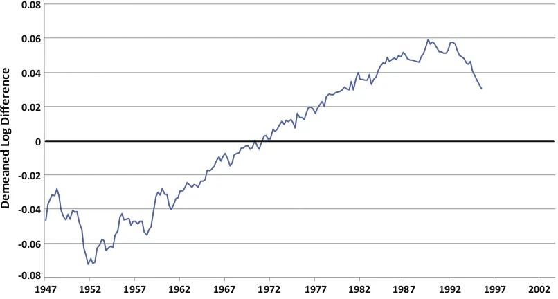
Figure 3. Stark plot across January 1996 benchmark revision. The plot shows the demeaned log differences of GDP before and after the benchmark revision of January 1996. It is a plot of log[X(t,b)/X(t,a)] –m, whereX(t,s) is the level ofXat datetfrom vintages, wheres=aors =b,b>a, andmis the mean of log[X(τ,b)/X(τ,a)] for all the dates that are common to both vintagesaandb. In this plot,a=December 1995 andb=October 1999. (Color figure available online.)

than other tests, including the standard Mincer–Zarnowitz test and the test for zero-mean forecast errors.

To conclude, this article by Patton and Timmermann provides us with an excellent set of tests that can complement much existing research. The tests help us cross two dimensions of forecast rationality: horizon and real-time vintage. They could potentially help as well in the subsample dimension.

[Received April 2011. Revised August 2011.]

REFERENCES

Brown, B. W., and Maital, S. (1981), “What Do Economists Know? An Em-pirical Study of Experts’ Expectations,”Econometrica, 49, 491–504. [17]

Croushore, D. (2010), “An Evaluation of Inflation Forecasts From Surveys Using Real-Time Data,”B.E. Journal of Macroeconomics: Contributions, 10, 10. [17]

——— (2011), “Two Dimensions of Forecast Analysis,” Working Paper, Uni-versity of Richmond. [17]

Croushore, D., and Stark, T. (2001), “A Real-Time Data Set for Macroe-conomists,”Journal of Econometrics, 105, 111–130. [18,19]

Faust, J., Rogers, J. H., and Wright, J. H. (2005), “News and Noise in G-7 GDP Announcements,” Journal of Money, Credit, and Banking, 37, 403–419. [19]

Keane, M. P., and Runkle, D. E. (1990), “Testing the Rationality of Price Forecasts: New Evidence From Panel Data,”American Economic Review, 80, 714–735. [17]

Patton, A. J., and Timmermann, A. (2011), “Forecast Rationality Tests Based on Multi-Horizon Bounds,”Journal of Business and Economic Statistics, this issue. [18]

Zarnowitz, V. (1985), “Rational Expectations and Macroeconomic Forecasts,” Journal of Business & Economic Statistics, 3, 293–311. [17]

Comment

Kajal L

AHIRI

Department of Economics, University at Albany: SUNY, Albany, NY 12222 (klahiri@albany.edu)

1. INTRODUCTION

I enjoyed reading yet another article by Patton and Timmer-mann (PT hereafter) and feel that it has broken new ground in testing the rationality of a sequence of multi-horizon fixed-target forecasts. Rationality tests are not new in the forecasting literature, but the idea of testing the monotonicity properties of second moment bounds across several horizons is novel and can suggest possible sources of forecasting failure. The basic premise is that since fixed-target forecasts at shorter horizons

are based on more information, they should on the average be more accurate than their longer horizon counterparts. The inter-nal consistency properties of squared errors, squared forecasts, squared forecast revisions, and the covariance between the tar-get variable and the forecast revision are tested as inequality

(3)

constraints across horizons. They also generalize the single-horizon Mincer-Zarnowitz (MZ) unbiasedness test by estimat-ing a univariate regression of the target variable on the longest horizon forecast and all intermediate forecast revisions. Using a Monte Carlo experiment and Greenbook forecasts of four macro variables, PT show that the covariance bound test and the gen-eralized MZ regression using all interim forecast revisions have good power to detect deviations from forecast optimality. I am sure we will be using, extending, and finding caveats with some of the testing proposals suggested in this article for years to come.

2. THEORETICAL CONSIDERATIONS

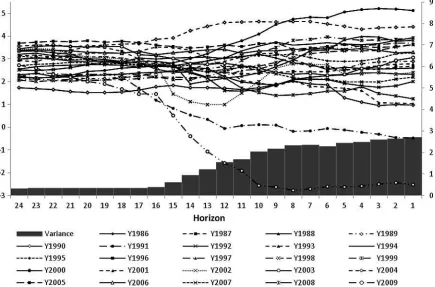
An important starting point of the article is that for internal consistency of a sequence of optimal forecasts, the variance of forecasts should be a weakly decreasing function of the forecast horizon. This point has been discussed by Isiklar and Lahiri (2007), and was originally the basis for testing whether data re-visions are news (and not noise) by Mankiw and Shapiro (1986). In order to highlight the nature of the fixed-target forecast vari-ances, I have plotted inFigure 1the sequences of monthly real GDP forecasts for 24 target years 1986–2009 from horizons 24 to 1 using consensus forecasts from the Blue Chip surveys. This survey is very well suited to examining the dynamics of forecasts over horizons. The respondents start forecasting in January of the previous year, and their last forecast is reported at the beginning of December of the target year. The shaded bars in the bottom ofFigure 1are the variances of mean fore-casts calculated over the target years. Clearly, the variances are nondecreasing functions of horizons and thus the relationship is consistent with rational expectations. Isiklar and Lahiri (2007) explained the relationship by the following logic. Consideryt

=ft,h+ ut,h where yt is the actual GDP growth, ft,h is theh

-period ahead forecast (h=24, 23,. . ., 1) made at timet–h, andut,h denotes the ex-post error associated with this forecast.

Since rational expectations imply that cov(ft,h,ut,h)=0, we have

var(yt)=var(ft,h)+var(ut,h), which implies (since for fixed

tar-get forecasts, variance ofytis same for allh) that the variations

in forecasts and forecast errors move in opposite directions as the forecast horizon changes. Therefore, as the forecast horizon decreases, the forecast error variability (and therefore the un-certainty) also decreases, but the forecast variability increases. Another way of looking at this increasing variability of fore-casts is that as the forecast horizon decreases, more information is absorbed in the forecasts, thus increasing their variability. This information accumulation process can be seen using a simple moving average (MA) data-generating process. Suppose that the actual process has a moving average representation of orderq so thatyt =µ+

q

k=0θkεt−kwith var(εt)=σ2. LetIt,hdenote

the information available at timet-h. Then, the optimal forecast at horizonhwill be

ft,h≡E(yt|It,h)=µ+ q

k=h

θkεt−k, (1)

and the variance of the forecast is

var(E(yt|It,h))=σ2 q

k=h

θ_k2. (2)

Similarly, the variance of the forecast when the forecast horizon is h – 1 is var(E(yt|It,h−1))=σ2

Thus, when the forecast horizon is very long, that is, sev-eral years, the forecasts tend to converge toward the mean of the process, and as information is accumulated, the forecasts change increasing the forecast variability.Figure 1exhibits this phenomenon very well. Note that for horizons from 24 to 16, the variance seems to remain constant, as was illustrated by Isiklar and Lahiri (2007) for a large number of countries, but with a smaller sample size using the Consensus Survey forecasts. The forecast variability increases because of the variability of the accumulated shocks, that is,θkεt−k. Therefore, if forecast

vari-ability does not change over several long horizons, this may mean that the information acquired at 24 to 16 horizons does not have much impact on the actual value, that is,|θk|is small

or equivalently relevant information simply does not exist. Of course, this may also be related to the informational inefficiency of the forecasts. It is possible that even if potentially relevant information over these horizons were available, the forecast-ers did not incorporate them appropriately causing less than optimal variability in the forecasts. The point here is that due to the nonmonotone arrival and use of information by forecast-ers at different horizons, the monotonicity properties of second moments like the forecast variance that PT exploit may be less obliging for the detection of forecast suboptimality.

The first difference in the MSEh provides a measure of the

new information content of forecasts when the horizon ish. On the basis ofEquation (1), an optimal forecastft,hsatisfies

MSE(ft,h)≡MSE(ft,h+1)−MSE(ft,h)=θh2σ

2_,

(3)

which is equivalent to the information content of the new infor-mation in the actual process.

Now let ˜It,hdenote a strict subset ofIt,h, and ˜ft,hbe a

subop-timal forecast, which is generated according to

˜

where q denotes the longest forecast horizon at which the first fixed-target forecast is reported—it defines the conditional mean of the actual process when the horizon is q, that is,

˜

µ=E(yt|I˜t,q); ˜εt−hdenotes the “news” component used by the

forecaster, and ˜θhdenotes the impact of this news component as

perceived by the forecaster.

For convenience, let us assume that the forecasters observe the newsεt−hcorrectly, but that their utilization of news is not

optimal, so that ˜θh=θhand ˜εt−h=εt−h. Thus, we see that the

where the first component on the right-hand side (RHS) de-notes the bias in the forecast, the second component dede-notes the error due to inefficiency, and the third component denotes the error due to unforecastable events after the forecast is re-ported. Calculating mean squared error (MSE) and assuming that sample estimates converge to their population values, we

(4)

Figure 1. Evolution of fixed target forecasts over horizons and their variances.

get

MSEh=(µ−µ˜)2+ q

k=h

(θk−θ˜k)2σ2+ h−1

k=0

θ_k2σ2. (6)

Thus, we find thatMSEh≡MSEh+1−MSEhis MSEh=θh2σ

2

−(θh−θ˜h)2σ2, (7)

which gives the improvement in forecast content with the new information. The first element on the RHS represents the max-imum possible improvement in the quality of forecasts if the information is used efficiently, but the second component rep-resents the mistakes in the utilization of the new information. If the usage of the most recent information ˜θhdiffers from its

op-timal valueθh, the gain from the utilization of new information

will decrease and result in excess variability in the forecasts given by the second term. In the special case where ˜θh=θh,

Equation (7)is equivalent toEquation (3). In this case,MSEh

will measure the content of new information in the actual process, which is simply θ2

hσ

2_{. Note, however, that a}

non-negative MSE differential is compatible with the situation where ˜

θh=θhfor a wide range of parameter values. This underscores

the point that the bounds derived by PT are implied by fore-cast rationality, and hence are not necessary conditions. In other words, if these tests reject the null, we have evidence against forecast rationality, but if the tests do not reject, we cannot say we have evidence in favor of rationality. The issue is whether ex-tant forecast efficiency tests, like those due to Nordhaus (1987) or Davies and Lahiri (1999), would detect forecast irrationality under the latter scenario.

While the use ofMSEh provides an estimate of the

im-provement in forecasting performance at horizonhin an ex-post sense, a similar measure can be constructed based solely on forecasts without using the actual data on the target variable—a point emphasized by PT. Notice that, based on Equation (1), the optimal forecast revisionrt,h≡ft,h−ft,h+1is nothing but

rt,h=θhεt−h. In the suboptimal case ofEquation (4), we have

the forecast revision processrt,h=θ˜hεt−h. Calculating the mean

squared revisions (MSRs) at horizonhand taking the probability limit, we get MSRh=plimT _T1 Tt=1rt,h2 =θ˜h2σ2, which

pro-vides a measure for the reaction of the forecasters to news. But since forecasters react to news based on their perceptions of the importance of the news, this measure can be seen as the content of the new information as perceived by the forecasters in real time. Note the clear difference between MSEh and MSRh. While the former is driven by the forecast errors, the

latter has nothing to do with the actual process or the outcomes. But both of the measures should give the same values if the survey forecasts are optimal. This result was originally pointed out by Isiklar and Lahiri (2007).

The difference between MSRhandMSEhmay provide

im-portant behavioral characteristics of the forecasters such as over or underreaction to news at a specific forecast horizon. MSRh

can be seen as a measure of how forecasters interpret the im-portance of news at a specific horizon, andMSEhcan be seen

as the “prize” they get as a result of revising their forecasts. Suppose that forecasters make large revisions at horizonh, but the performance of the forecasts does not improve much at that horizon, then one may conjecture that the forecasters react ex-cessively to the news. To see this more clearly, simple algebra yields MSRh−MSEh=2( ˜θh2−θhθ˜h)σ2, which is positive

(5)

0 0.5 1 1.5 2 2.5 3

-0.05 0 0.05 0.1 0.15 0.2 0.25 0.3 0.35

23 22 21 20 19 18 17 16 15 14 13 12 11 10 9 8 7 6 5 4 3 2 1

Horizon

MSE MSR MSE PT’s MSR

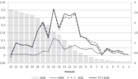
Figure 2. MSE, MSF, and their differentials, Blue Chip Consensus Forecasts 1986–2009.

when ˜θ2

h > θhθ˜h. This is the same as the condition|θ˜h|>|θh|.

But|θ˜h|>|θh|is equivalent to overreaction to the news when

the horizon ish. Thus, forecast optimality can be tested by the equality between MSRh andMSEh. This concept is the

ba-sis of the amended Nordhaus-type rationality test suggested by Lahiri and Sheng (2008) in which forecast error is regressed on the latest forecast revision for testing its significance. Note that PT’s bounds test on the MSRs is defined slightly differently as the difference betweenft,1−ft, mandft,1−ft, m−1wheremis an

intermediate horizon.

3. ADDITIONAL SURVEY EVIDENCE

In order to visualize the differences in MSRhas we defined

above,MSEhand PT’s MSR, we plotted these values in

Fig-ure 2, calculated from the Blue Chip consensus forecasts over

1986–2009. The actual values are the first available real-time data obtained from the Philadelphia Fed’s real-time database. First note that PT’s MSR andMSEh are almost identical at

most horizons because when the shortest horizon forecast is very close to the actual value, as is actually the case, the two mea-sures will be very similar. Second, both are nonnegative at all horizons suggesting forecast rationality by the PT criteria. How-ever, we find a substantial wedge between MSRhandMSEh

particularly in the middle horizons that suggests substantial un-derreaction to news, and hence inefficiency. Thus, PT’s MSE and MSR differential bounds conditions are not stringent enough to detect inefficiency in the Blue Chip consensus forecasts. This is consistent with the evidence they report. Note, however, with the same Blue Chip data series over 1977–2009, the Nordhaus test readily rejects rationality over multiple horizons with adjusted R2in excess of 0.20 and the coefficient on the lagged forecast revision around 0.58. This result is valid over different sample periods 1977–2009 and 1986–2009, over all horizons and also

over horizons between 16 and 6. Note that even though PT did not consider the Nordhaus test in their experiments, their bounds test that the variance of the forecast revision should not exceed twice the covariance between the forecast revision and the ac-tual value is effectively the Nordhaus test in disguise because, given that the longer horizon forecasts have larger MSEs than shorter horizon forecasts, this particular PT condition is derived using the Nordhaus condition that forecast errors should be un-correlated with forecast revisions under forecast efficiency (see their proof of Corollary 4 in the appendix).

We also experimented with the extended MZ regression us-ing consensus Blue Chip real GDP forecasts from 1977 to 2009. Data on horizons 16 through 7 are available throughout the Blue Chip sample. PT’s univariate optimal revision regression gen-eralizing the MZ regression rejected the null that the intercept is zero and that the coefficients of the horizon 16 forecast and the series of intermediate forecast revisions are one with the p-value of 0.07. But all individual MZ regressions accepted the unbiasedness hypothesis withp-values in excess of 0.5. This re-sult is very similar to what PT found with Greenbook forecasts on real GDP. However, the high multicollinearity between suc-cessive revisions tends to make this regression highly unstable, particularly when forecasts on a large number of horizons are available. Thus, one should be careful while using this test—the conclusions using this test may depend on the horizons included in the extended regression.

I also used another rich survey panel dataset—the U.S. Survey of Professional forecasters (SPF)—over 1968Q4–2011Q1 using three primitive forecasts of individuals (ID nos 40, 65, and 85) each having more than 100 quarters of participation, and also all forecasters who participated at least 10 times yielding a total of 425 forecasters in the “all” group. I used real GDP forecasts for six available horizons—beginning with the current quarter. Various forecast statistics are reported inTable 1. The actual

(6)

Table 1. Real GDP forecast error statistics for SPF data

Forecaster ID no. 40 Forecaster ID no. 65 Forecaster ID no. 85 All

Horizon quarter MSE MSR MSE MSE MSR MSE MSE MSR MSE MSE MSR MSE

1 7.295 2.997 0.788 4.447 5.645 4.62 4.572 2.283 2.66 7.083 7.203 3.793 2 8.083 1.765 3.442 9.067 2.962 2.066 7.232 1.789 −0.789 10.876 6.650 2.444 3 11.525 0.766 1.147 11.133 2.927 0.474 6.443 1.326 −0.148 13.320 6.696 3.543 4 12.672 1.495 −4.129 11.607 4.934 3.69 6.295 2.142 5.057 16.863 5.601 −0.065

5 8.543 - - 15.297 - - 11.352 - - 16.798 -

-GDP values are again the real-time figures released one month after the end of the quarter. Here, we find very few negative MSEhor MSR values that would suggest inefficiency. Only

the MSE differential for forecaster 40 between quarter 5 and quarter 4 is substantially negative, suggesting forecast subopti-mality. However, this evidence of inconsistency can be a result of the arrival of the current year’s real GDP value for predicting the first quarter GDP growth for the next year. More generally, relevant information regarding different target values may ar-rive at different times in a nonmonotone manner, and as a result, the relative forecast accuracy over horizons may not be smooth. PT’s approach of pooling all horizons together to test forecast rationality can mask this important horizon-specific heterogene-ity in forecast efficiency. In other words, forecasts may be effi-cient at certain horizons but not at others.

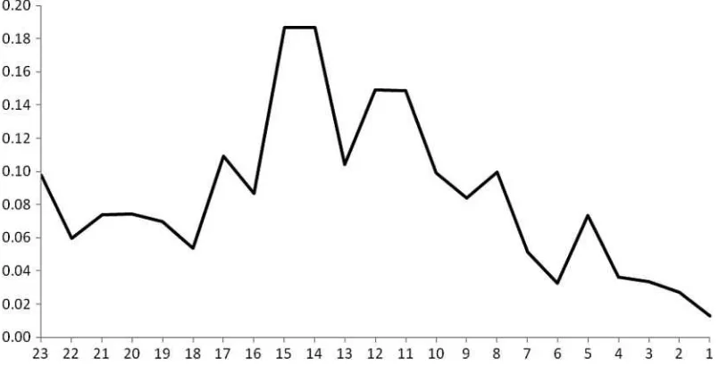
In Figure 3, we have plotted total sum of squares of

fore-cast revisions (defined as S_ht =Nh

i=1

ti h

t=1 (ri

t,h−

=

rh)2 Nh

i=1Thi

, where

i refers to the ith forecaster, r_t,hi =f_t,hi −f_t,hi ₊₁, =rh =

1

Nh

i=1 1

Ti h

t=1r

i

t,h, andNhandThidenote the available

obser-vations) at horizons from 23 to 1 to illustrate that the maximum amount of revisions take place in the middle horizons, and inter-estingly, the maximum amount of underreaction to news takes place at these horizons too. See Lahiri and Sheng (2010) for

additional evidence on this point. These results mean that the efforts put forward by forecasters to produce serious forecasts vary by horizons, and the process begins seriously at around 16-month horizon. Thus, forecasting efforts and the resulting efficiency are also conditioned by the institutions’ requirements under which the forecasters operate. To truly understand the forecasting inefficiencies, the demand side of the forecasting market should also be considered, in addition to the schedule of official data announcements.

There are a few more such negative (though small) MSE differentials inTable 1. PT also found a similar result with re-spect to Greenbook real GDP forecasts; see also Clements et al. (2007). We find that the MSE differentials and MSRs are quite different particularly in the middle horizons and the latter tend to underestimate the former, suggesting underreaction to new in-formation. Following PT, we also calculated MSR differentials betweenft,2−ft, 4andft,2−ft, 3, andft,3−ft, 5andft,3−ft, 4;

and betweenft,4−ft, 6andft,4−ft,5for the three long-standing

forecasters and also for the “all’ group using disaggregate data. In none of the cases did we find any evidence of negative MSR differentials and thus we fail to detect any indication of irra-tionality based on this MSR criterion. However, the Nordhaus test and the regressions of forecast errors on forecast revisions, a laLahiri and Sheng (2008,2010), readily detected deviations from rationality in most cases.

Figure 3. Total sum of squares in GDP forecast revisions during 1986–2009: Blue Chip Surveys.

(7)

4. CONCLUSION

I find the ideas put forward in this article to rigorously test the optimality of forecasts across horizons interesting and the efforts to implement the tests quite commendable. Despite their math-ematical elegance, these derived bounds are implied by forecast rationality, and hence are not necessary conditions. Thus, if the tests do not reject the null, we cannot say we have evidence in favor of rationality. For instance, even though the forecast vari-ances and MSEs are observed to be weakly decreasing functions of the forecast horizon, the underlying forecasts can be easily be still inefficient. By using Blue Chip and SPF survey fore-casts, we found, like PT, that some of the bounds tests proposed in the paper are not very powerful to detect suboptimality in instances where the extant Nordhaus test readily identifies it. However, their new extended MZ test based on a regression of the target variable on the long-horizon forecast and the se-quence of interim forecast revisions works well, provided the multicollinearity problem does not become serious. We have argued that by testing the equality of MSE differentials with mean square forecast revisions, one can also examine forecast rationality over multiple horizons. In order to truly understand the pathways through which forecasts fail to satisfy forecast op-timality, we have also to consider the demand side of the fore-casting market and the schedule of official data announcements. For instance, there is evidence that forecasters record maximum suboptimality at horizons where they also make maximum cast revisions. The observed suboptimality of Greenbook fore-casts that PT found cannot be understood unless the institu-tional requirements of such forecast are appreciated. Neverthe-less, the importance of testing the joint implications of forecast

rationality across multiple horizons when such information is available as proposed by the authors must be appreciated.

ACKNOWLEDGMENTS

The author thanks Antony Davies, Gultikin Isiklar, Huaming Peng, Xuguang Sheng, and Yongchen Zhao for many useful discussions and research assistance, and to the co-editors for making a number of helpful comments.

[Received June 2011. Revised July 2011.]

REFERENCES

Clements, C. P., Joutz, F., and Stekler, H. (2007), “An Evaluation of Forecasts of the Federal Reserve: A Pooled Approach,”Journal of Applied Econometrics, 22, 121–136. [24]

Davies, A., and Lahiri, K. (1999), “Re-examining the Rational Expectations Hypothesis Using Panel Data on Multi-period Forecasts,” in Analysis of Panels and Limited Dependent Variables, eds. C. Hsiao, K. Lahiri, L. F. Lee, and H. Pesaran, Cambridge, U.K.: Cambridge University Press, pp. 226–254. [22]

Isiklar, G., and Lahiri, K. (2007), “How Far Ahead can We Forecast? Evidence from Cross-country Surveys,”International Journal of Forecasting, 23, 167– 187. [21,22]

Lahiri, K., and Sheng, X. (2008), “Evolution of Forecast Disagreement in a Bayesian Learning Model,”Journal of Econometrics, 144, 325–340. [23,24] Lahiri, K., and Sheng, X. (2010), “Learning and Heterogeneity in GDP and Inflation Forecasts,” International Journal of Forecasting, 26, 265– 292. [24]

Mankiw, N. G., and Shapiro, M. D. (1986), “News or Noise? An Analysis of GNP Revisions,”Survey of Current Business, 66, 20–25. [21]

Nordhaus, W. (1987), Forecasting Efficiency; Concepts and Applications, Re-view of Economics and Statistics, 69, 667–674. [22]

Comment

Barbara R

OSSI

Department of Economics, 204 Social Science Building, Duke University, Durham, NC 27708, ICREA, and University Pompeu (brossi@econ.duke.edu)

Patton and Timmermann (2011) propose new and creative forecast rationality tests based on multi-horizon restrictions. The novelty is to consider the implications of forecast rationality jointly across the horizons. They focus on testing implications of forecast rationality such as the fact that the mean squared forecast error should be increasing with the forecast horizon (Diebold 2001; Patton and Timmermann 2007) and that the mean squared forecast should be decreasing with the horizon. They also consider new regression tests of forecast rationality that use the complete set of forecasts across all horizons in a univariate regression, which they refer to as the “optimal revi-sion regresrevi-sion” tests. One of the advantages of the proposed procedures is that they do not require researchers to observe the target variable, which sometimes is not clearly available. In fact, Patton and Timmermann (2011) show that both their in-equality results as well as the “optimal revision regression” test hold when the short horizon forecast is used in place of the target variable. Their work is an excellent contribution to the literature.

The main objective of this comment is to check the robust-ness of forecast rationality tests to the presence of instabilities. The existence of instabilities in the relative forecasting perfor-mance of competing models is well known [see Giacomini and Rossi (2010) and Rossi and Sekhposyan (2010), among others; Rossi (2011) provide a survey of the existing literature on forecasting in unstable environments]. First, we show heuris-tic empirical evidence of time variation in the rolling estimates of the coefficients of forecast rationality regressions. We then use fluctuation rationality tests, proposed by Rossi and Sekh-posyan (2011), to test for forecast rationality, while, at the same time, being robust to instabilities. We also consider a version of Patton and Timmermann’s (2010) optimal revision