Full Terms & Conditions of access and use can be found at
http://www.tandfonline.com/action/journalInformation?journalCode=ubes20
Download by: [Universitas Maritim Raja Ali Haji] Date: 11 January 2016, At: 23:07
Journal of Business & Economic Statistics
ISSN: 0735-0015 (Print) 1537-2707 (Online) Journal homepage: http://www.tandfonline.com/loi/ubes20
Local and Global Rank Tests for Multivariate
Varying-Coefficient Models
Stephen G. Donald, Natércia Fortuna & Vladas Pipiras
To cite this article: Stephen G. Donald, Natércia Fortuna & Vladas Pipiras (2011) Local and Global Rank Tests for Multivariate Varying-Coefficient Models, Journal of Business & Economic Statistics, 29:2, 295-306, DOI: 10.1198/jbes.2010.07303
To link to this article: http://dx.doi.org/10.1198/jbes.2010.07303
Published online: 01 Jan 2012.
Submit your article to this journal
Article views: 109
Local and Global Rank Tests for Multivariate
Varying-Coefficient Models
Stephen G. D
ONALDDepartment of Economics, University of Texas at Austin, Austin, TX 78712 (donald@eco.utexas.edu)
Natércia F
ORTUNACEF.UP, Faculdade de Economia, Universidade do Porto, Rua Dr. Roberto Frias, 4200-464 Porto, Portugal (nfortuna@fep.up.pt)
Vladas P
IPIRASCEMAT, Instituto Superior Técnico, Lisbon 1049-001, Portugal and Department of Statistics and Operations Research, University of North Carolina at Chapel Hill, Chapel Hill, NC 27599 (pipiras@email.unc.edu)
In a multivariate varying-coefficient model, the response vectorsYare regressed on known functions
v(X)of some explanatory variablesXand the coefficients in an unknown regression matrixθ(Z)depend on another set of explanatory variablesZ. We provide statistical tests, called local and global rank tests, which allow one to estimate the rank of an unknown regression coefficient matrixθ(Z)locally at a fixed level of the variableZor globally as the maximum rank over all levels ofZin a proper, compact subset of the support ofZ, respectively. We apply our results to estimate the so-called local and global ranks in a demand system where budget shares are regressed on known functions of total expenditures and the coefficients in a regression matrix depend on prices faced by a consumer.
KEY WORDS: Demand systems; Kernel smoothing; Local and global ranks; Matrix rank estimation; Varying-coefficient model.
1. INTRODUCTION
1.1 Statement of the Problem
Let(Xi,Zi)∈Rp×Rqbe independent variables,Yi∈Rmbe
response variables, andUi∈Rm be error terms. The focus of
this work is on the statistical model
Yi=(0(Zi) (Zi) ) V
0(Xi)
V(Xi)
+Ui
=θ(Zi)v(Xi)+Ui, i=1, . . . ,N, (1.1)
whereNis the number of observations,θ(z),0(z), and(z)
are unknownm×n,m×d0, andm×dmatrices of functions
ofz, respectively, andv(x),V0(x), andV(x)are knownn×1,
d0×1, andd×1 vectors of functions of x, respectively. We partition the matrixθ(z)into two submatrices0(z)and(z)
because we will work with the matrix(z). Whend0=0, we suppose by convention that0(z)is empty and hence focusing
on(z)is more general than working with the matrixθ(z). In applications to demand systems below, in particular, we shall supposed0=0 and be interested in the matrix(z)alone. Note
also that
(z)=θ(z)
0 d0×d
Id
=:θ(z)α. (1.2) (The matrixαwill be used below.) Important assumptions on the model (1.1) are smoothness of the functions of θ(z) and nonsingularity of the covariance matrix
=EUiU′i. (1.3)
The rest of the assumptions can be found in Section2.
The model (1.1) and its slight variants, generally known as varying-coefficient models, were considered by Cleveland,
Gross, and Shyu (1991), Hastie and Tibshirani (1993), Fan and Zhang (1999, 2000, 2008), Cai, Fan, and Li (2000), Fan, Zhang, and Zhang (2001), Li et al. (2002), Wang (2008), and others in the context of regression, longitudinal analysis, and nonlin-ear time series. It is also covered in a recent comprehensive monograph on nonparametric methods by Li and Racine (2007, chapter 9). Extensions of the model, such as a partially linear varying coefficient model, are studied in Xia, Zhang, and Tong (2004), Ahmad, Leelahanon, and Li (2005), Fan and Huang (2005), Lu (2008), and others. Some of the considered appli-cations include cases whereY,X, andZare, respectively, hos-pital admissionsY, level of pollutantsX, and timeZ(Fan and Zhang1999, 2000); value addedY, value of capital assets and number of employeesX, and intermediate production and man-agement expenseZ in a production function (Li et al.2002); median value of owner-occupied homeY, per capita crime rate and other variables X, and a particular index variableZ in a Boston housing data (Wang2008).
Several estimation methods for the functions of θ(z)have been proposed. A simple and common choice is a kernel-based estimator
θ(z)= 1
Nhq N
j=1
Yjv(Xj)′K z
−Zj
h
×
1
Nhq N
j=1
v(Xj)v(Xj)′K z
−Zj
h
−1
, (1.4)
© 2011American Statistical Association Journal of Business & Economic Statistics April 2011, Vol. 29, No. 2 DOI:10.1198/jbes.2010.07303
295
whereK is a kernel function andh>0 is a bandwidth. More sophisticated methods can be based on local polynomial regres-sion but will not be considered here for simplicity (Fan and Gi-jbels1996; Li and Racine2007).
In this work, we are interested in the model (1.1) with several related objectives in mind. Let rk{A}denote the rank of a matrix A. One of our goals is to address the hypothesis testing prob-lem ofH0: rk{(z)} ≤ragainstH1: rk{(z)}>r, whererand
zare fixed. The problem of testing for the rank of a matrix is well studied. In the linear regression context, it goes back to An-derson (1951). Other general and commonly used methods are based on the Lower-Diagonal-Upper triangular decomposition (Gill and Lewbel1992; Cragg and Donald1996), the minimum-χ2test statistic (Cragg and Donald1993, 1996, 1997), the sin-gular value decomposition (Kleibergen and Paap2006), or the idea of the Asymptotic Least Squares (Robin and Smith1995). These methods require the asymptotic normality of an estimator of the matrix. As we show, under suitable conditions, the esti-mator(z)based on (1.4) is asymptotically normal and hence the aforementioned methods can be applied directly. Sincezis fixed, the statistical tests for the rank of the matrix(z)will be calledlocal rank tests.
We shall also address the problem ofglobal rank tests, that is, the hypothesis testing problem ofH0: supzrk{(z)} ≤ragainst
H1: supzrk{(z)}>r, whereris fixed and the supremum is taken over a proper, compact subset of the support of Z. This problem has not been previously considered to our knowledge. Global rank tests will be based on the statistic obtained by inte-grating the minimum-χ2statistic of the local rank tests over the range of values ofz. Establishing the asymptotics of the result-ing global test statistic is quite involved because the minimum-χ2 statistic is a nonlinear functional of(z). In fact, we are not able to find the exact limit of the global test statistic under
H0. We only show that the statistic is asymptotically bounded (stochastically dominated) by the standard normal law. Despite this simplification, a number of new theoretical difficulties had still to be overcome. Moreover, since we expect the exact limit to be nonstandard (and bounded by the standard limit law), our asymptotic result is quite sufficient from a practical perspective. It should also be added here that (local and global) rank tests lead naturally to estimates of the rank of a matrix itself. One typical way to do this is through a sequential testing where the above hypothesis tests are performed for increasing integers
r=0,1, and so on, till the first time the hypothesisH0cannot
be rejected. (For a reader little familiar with these problems, note also that the matrix rank cannot be estimated by that of its estimator. Because of the noise term in the model and from a practical perspective, the estimator is typically of full rank itself.)
1.2 Economic Motivation
Our other goal is to apply the obtained local and global rank tests to a demand system. In the context of demand systems,Yi
are budget shares forjgoods,Xiare total expenditures (income,
in short), andZiare prices ofjgoods faced by theith consumer.
The corresponding varying-coefficient model is
Yi=θ(Zi)v(Xi)+ǫi, i=1, . . . ,N, (1.5)
where, similarly to (1.1),θ(z)is a j×n matrix of unknown functions andv(x)is an×1 vector of known functions. The models (1.5) represent the class of deterministic demand sys-temsy=f(x,z)=θ(z)v(x)known asexactly aggregable de-mand systems. These demand systems are important in Eco-nomic Theory since they have nice theoretical properties, for example, related to aggregation and representative consumer (Muellbauer1975, 1976; Gorman1981; and others), and also since they encompass many well-known examples of demand systems, for example, AIDS, translog, PIGL, and others, as their special cases. They have been also widely used in applica-tions (Hausman, Newey, and Powel1995; Banks, Blundell, and Lewbel1997; Nicol2001; and others).
An important departure from the earlier statistical works on demand systems is that we allow the coefficient matrixθto de-pend on price variables. Most of the authors exclude variation in prices for simplicity and also because commonly used data sets of demand systems, for example, the Consumer Expendi-ture Surveys (CEX, in short) dataset for the United States, does not contain information on prices. The assumption of constant prices is not realistic. We shall use the CEX dataset and as-sign prices to its households by drawing prices from the Ameri-can Chamber of Commerce Research Association (ACCRA, in short) dataset and by using some location variables in the CEX dataset as matching variables. It can be seen from the ACCRA dataset that prices are quite different across the United States.
We are interested in estimation of rk{θ(z)}and supzrk{θ(z)}. Following Lewbel (1991), alocal rank atzof a demand system
y=f(x,z)=(f1(x,z), . . . ,fj(x,z))′is defined as the dimension
of the function space spanned by the coordinate functions of f(x,z)for fixedz. Aglobal rankof a demand system is defined as the maximum of local ranks over all possible values of z. It involves simple algebra to see that a local rank rk{f(·,z)}of the exactly aggregable demand systemy=f(x,z)=θ(z)v(x) is equal to rk{θ(z)} when v(x) consists of linearly indepen-dent functions of x (Proposition B.1 below). Some theoreti-cal studies on ranks can be found in Gorman (1981), Lewbel (1991, 1997), and others. In particular, Gorman (1981) showed that exactly aggregable demand systems, when derived through a utility maximization principle, have always rank less than or equal to 3.
To estimate rk{θ(z)} and supzrk{θ(z)}, observe, however, that one cannot readily apply the local and global rank tests un-der the model (1.1). Since the elements ofYiare budget shares,
they add up to 1 and hence the covariance matrix ofǫi is
sin-gular whereas that of Ui in (1.3) is assumed nonsingular. To
avoid singularity, one commonly drops one share of goods from the analysis which allows one to assume a nonsingular covari-ance matrix of the reduced error terms. To estimate rk{θ(z)}, it is then necessary to be able to relate rk{θ(z)}to some char-acteristic of the matrixθ(z) with one row eliminated. When v(x)=(1V(x)′)′as typically assumed in practice, we have that rk{θ(z)} =rk{(z)} +1, (1.6) where(z)is the matrixθ(z)with an arbitrary row and the first column eliminated (see PropositionB.1below). In view of this relation, we will therefore eliminate one budget share from
assuming that the covariance matrix ofUi is nonsingular, and
then obtain estimates of rk{θ(z)}and supzrk{θ(z)}by adding 1. We shall apply this estimation procedure to estimate local and global ranks in the demand system constructed from the CEX and the ACCRA data sets. Related estimation of local ranks in a demand system given by a nonparametric model can be found in Fortuna (2008).
1.3 Outline of the Article
The rest of the article is organized as follows. In Section2, we state the assumptions which are used in connection to the model (1.1). In Section3, we introduce an estimator for the ma-trix(z)based on (1.4) and, in particular, state its asymptotic normality result. Local and global rank tests for the matrices (z)are studied in Sections4and5, respectively. Simulation experiment is presented in Section6. Estimation of local and global ranks in a demand system can be found in Section7. Some proofs are postponed till AppendicesAandB.
2. ASSUMPTIONS AND OTHER NOTATION
We shall use the following assumptions on the variablesXi,
Zi, andUi, on the functionsθandv, and on the kernelK.
Assumption 1. The functionKis a symmetric kernel onRq
of orders, that is, K has a compact support, is bounded and satisfies the following conditions: (i) RqK(z)dz=1 and (ii)
There are many possible choices for such kernelsK. In the simulation experiment and the application below, whenq=1, we use the popular Epanechnikov kernelK(z)=3(1−z2)/4, for |z| ≤1, of the order s=2. The kernel K(z)=15(7z4−
10z2+3)/32, for |z| ≤1, of the order s=4, is another pos-sibility. For a given kernelK, we shall also use the following related kernels throughout the article: (the so-called convolution kernel). The notation Kh(z) will
stand for a scaled kernel h−qK(z/h).We shall also use obvi-ous combinations of the notation above such asK2,hand so on.
Assumption 2. Suppose that(Xi,Zi)∈Rp×Rq,i=1, . . . ,
N, are iid random vectors such that the supportHzofZiis the
Cartesian product of compact intervalsHz= [a1,b1] × · · · ×
[ap,bq]andZi is continuously distributed with a densityp(z).
Suppose that the densityp(z)hasscontinuous bounded deriv-atives onHz, and that p(z)is bounded away from zero in the interior ofHz.
Assumption 3. Suppose that the error termsUi,i=1, . . . ,N,
are iid random vectors, independent of the sequence (Xi,Zi)
and such thatEUi=0and
EUiU′i=, (2.3)
whereis am×mpositive definite matrix. Suppose also that
E|Ui|u<∞whereu≥4.
Local rank tests can also be obtained under a weaker, het-eroscedasticity assumption onUi, that is,E(UiUi′|Xi=x,Zi=
z)=(x,z). Under the stronger condition (2.3), the limit co-variance matrix in the asymptotic normality result forθ(z)has a convenient Kronecker product structure. The proof of the global rank tests uses this Kronecker product structure and hence the stronger condition (2.3). Regarding Assumption 2, the condi-tion of bounded support ofZican be removed by requiring
fi-nite suitable moments of functionsψkdefined below.
Assumption L4. In the case of local rank tests, the function θ:Hz→Rmnis such that each of its component functions has
scontinuous derivatives onHz.
Assumption G4. In the case of global rank tests, suppose that the component functions ofθ(z)are real analytic onHz(see the discussion below).
Assuming smoothness (i.e., continuity of derivatives of some order) of the function θ(z)is standard for varying-coefficient models (see the references provided in Section 1.1). The as-sumption of analyticθ(z)for global rank tests is less common and requires further explanation. According to one possible de-finition, a function f is analytic if its Taylor series converges to the function fat a neighborhood of each point. We assume analyticity just in order to have smoothness of the eigenvectors of some analytic matrices involvingθ(z). It is well known that smoothness of a matrix is not sufficient to have smooth eigen-vectors (see, e.g., Kato1976; Bunse-Gerstner et al.1991).
To state the next assumptions, let
φk(z)=E(v(Xi)v(Xi)′)k|Zi=z
=:ψk(z)p(z)−1, k=1,2,4, (2.4) where, for a matrixA, we writeA2=AA′andA4=A2(A2)′. We writeφandψ forφ1andψ1, respectively.
Assumption L5. The matrixφ(z)is positive definite, and has
scontinuous derivatives onHz. The matricesφ2(z),φ4(z)are
continuous onHz.
Assumption G5. In the case of global rank tests, suppose in addition that the components ofψ(z)are real analytic.
If v(x)=(v1(x), . . . ,vn(x))′, the conditions on φ2(z) and
φ4(z)in AssumptionL5are effectively those on
E
wherei1, . . . ,i8are arbitrary indices from 1, . . . ,n. In addition
to (2.4), we shall also use thed×dmatrix (z)such that (z)−1=α′ψ(z)−1α, (2.5) whereαis defined in (1.2). Observe that, if the matrixψ(z)is positive definite, then (z)is positive definite and, ifψ(z)is real analytic, then (z)is also real analytic.
The global rank tests will be constructed over a subsetHof
Hzsatisfying the following assumption.
Assumption G6. Suppose thatHis a proper, compact subset ofHz.
The condition on properness in Assumption G6 is neces-sary to avoid boundary effects when using kernel smoothing. A number of boundary corrections are available (conveniently summarized in Karunamuni and Alberts2005) but using them here would unnecessarily complicate the technical level of the article. Moreover, in simulations reported below, our global rank test appears to work quite well even ignoring the boundary issue.
Assumption G7. Suppose thatq=1,2, or 3.
As seen from the proofs for global rank tests, the global rank test statistic has a leading bias term of the orderh2−q/2. The bias term is thus negligible only under AssumptionG7, and would have to be corrected properly in higher dimensionsq.
3. KERNEL–BASED ESTIMATOR
LetKbe a kernel defined in Assumption1of Section2. We shall use throughout a kernel-based estimatorθ(z)for the ma-trixθ(z)defined by (1.4). The estimatorθ(z)can also be ex-pressed as
θ(z)=YDzv′(vDzv′)−1=: 1
NYDzv
′ψ(z)−1, (3.1)
where Y=(Y1 · · · YN),v=(v(X1) · · · v(XN) ), and
Dz=diag{Kh(z−Z1), . . . ,Kh(z−ZN)}. A more general
esti-mator forθ(z)can be defined based on the idea of local polyno-mial regression (Fan and Gijbels1996; Fan and Zhang1999). We work with the estimator (3.1) for proof simplicity, espe-cially in the context of global rank tests.
Define the estimator(z)for the submatrix(z)ofθ(z)by using (1.2) as (z)=θ(z)α. The following result establishes the asymptotic normality of (z). The proof is standard and can be found in Donald, Fortuna, and Pipiras (2010).
Theorem 1. Under Assumptions 1–3,L4–L5of Section2, we have, for fixedzin the interior ofHz,
√
Nhqvec((z)−(z))→
dN(0,(z)), (3.2)
as
N→ ∞, h→0, Nhq→ ∞ and Nhq+2s→0, (3.3)
with
(z)=( (z)−1⊗)K22, (3.4)
where the matrix (z)is defined by (2.5). Suppose in addition that N1−2/uhq/lnN→ ∞ whereu appears in Assumption3. Then, the limiting covariance matrix(z)in (3.4) can be esti-mated consistently by
(z)=((z)−1⊗)K22, (3.5) where(z)−1=α′ψ(z)−1α withψ(z)−1 appearing in (3.1),
and
= 1
NpH N
i=1
(Yi−θ(Zi)v(Xi))
×(Yi−θ(Zi)v(Xi))′1{Zi∈H} (3.6) with H satisfying Assumption G6,pH=N−1Ni=11{Zi∈H} and 1Adenoting an indicator function.
Remark 1. Under slightly different assumptions, includ-ing the heteroscedasticity assumption E(UiU′i|Xi =x,Zi =
z) = (x,z), the asymptotic normality result for θ(z) is also proved in Li et al. (2002) (see also theorem 9.3 in Li and Racine 2007). The resulting covariance matrix is ψ(z)−1E(v(Xi)v(Xi)′(Xi,Zi)|Zi = z)ψ(z)−1K22 in the
casem=1.
The restriction ofZitoHappears in (3.6) for simplicity in
or-der not to deal with the boundary effects in the proofs. It is quite likely that the restriction can be removed but at the expense of a significant expansion of the proof. At least from a practical perspective, we do not see much difference in our simulations between using and not using the restriction toH.
4. LOCAL RANK TESTS
We consider here the hypothesis testing problem of H0:
rk{(z)} ≤ragainstH1: rk{(z)}>r,wherezandrare fixed.
Since(z)is an asymptotically normal estimator of(z)and the related covariance matrix (z) can be consistently esti-mated by(z)in (3.5) (Theorem1), this problem can be read-ily addressed by one of the rank tests available in the literature. Four such tests, mentioned in Section1.1, are the LDU-based test, the minimum-χ2, the SVD-based test and the ALS-based test. We recall below the minimum-χ2test only because its in-tegrated version will be used for global rank tests.
Minimum-χ2rank test. Applied to the matrix(z)with the covariance matrix(z), the minimum-χ2test is based on the statistic
T(r,z)=Nhq min
rk{}≤rvec(
(z)−)′(z)−1vec((z)−)
=NhqK−22
m−r
i=1
λi(z), (4.1)
where 0≤λ1(z)≤ · · · ≤λm(z)are the ordered eigenvalues of
the matrix
Ŵ(z)=−1(z)(z)(z)′. (4.2) The last equality in (4.1) is standard for the covariance matrix
(z)having a Kronecker product structure, and can be proved as, for example, theorem 3 in Cragg and Donald (1993). For the same covariance matrix (z), the test statistic (4.1) also coincides with that used in the SVD-based rank test.
The next result follows from Cragg and Donald (1997) and Robin and Smith (2000). In the context of linear regression, it goes back to Anderson (1951). LetYa×b be aa×bmatrix
with independent N(0,1) entries and set Xa,b=Ya×bYa′×b.
Let alsoλ1(Xa,b)≤ · · · ≤λa(Xa,b)be the ordered eigenvalues
of the matrixXa,b. The notationχ2(k)below stands for aχ2
-distribution withkdegrees of freedom, and a stochastic domi-nanceξ ≤dηmeans thatP(ξ >x)≤P(η >x)for allx∈R.
Theorem 2. Under the assumptions of Theorem1, we have: (i) whenr<rk{(z)},
lim(p)T(r,z)= +∞, (4.3) (ii) whenr≥rk{(z)} =:l(z),
lim(d)T(r,z) = m−r
i=1
λi
Xm−l(z),d−l(z)
≤dχ2((m−r)(d−r)), (4.4)
where the inequality ≤d becomes the equality =d for r =
rk{(z)}.
Theorem2can be used to test forH0: rk{(z)} ≤ragainst
H1: rk{(z)}>r in a standard way. The resulting local rank
tests can be used to estimate rk{(z)}, for example, by using a sequential testing procedure (see, e.g., Donald1997; Robin and Smith2000).
5. GLOBAL RANK TESTS
We are interested here in global rank tests, that is, the hy-pothesis testing problem of H0: supz∈Hrk{(z)} ≤r against
H1: supz∈Hrk{(z)}>r, whereris fixed andHis as in As-sumptionG6. LetT(r,z)be the minimum-χ2statistic defined by (4.1) and used in the local rank tests. In view of Theorem2, for global rank tests, it is natural to consider a test statistic based on
H
T(r,z)dz. (5.1)
The idea here is that, underH0, the term (5.1) is expected to be
Op(1), and underH1, it is expected to converge to+∞in
prob-ability. [Instead of (5.1), other global characteristics could be considered such as maxz∈HT(r,z)and, in fact, could be dealt with in the same way as (5.1) by a “linearization” argument em-ployed in the proof of global rank tests below.] A more precise asymptotics of (5.1) needs to take into account proper centering and normalization. Hence, consider
Tglb(r)= H
T(r,z)dz− |H|(m−r)(d−r)
hq/2|H|1/2√2(m−r)(d−r)
K22
K2 (5.2)
with|H| = Hdz, which will play the role of the global rank test statistic.
The next result establishes the asymptotics of the statistic
Tglb(r). We write lim sup(d)ξ≤dηif lim supP(ξ >x)≤P(η >
x)for allx∈R.
Theorem 3. Under the Assumptions 1–3, G4–G7 of Sec-tion2, and when
Nh2q/ln3N→ ∞, N1−2/uhq/lnN→ ∞, (5.3)
Nhq/2+s→0, we have:
(i) whenr<supz∈Hrk{(z)},
lim(p)Tglb(r)= +∞, (5.4)
(ii) whenr≥supz∈Hrk{(z)},
lim sup(d)Tglb(r)≤dN(0,1), (5.5)
where lim sup becomes lim and the inequality≤dbecomes the
equality=dwhenr=rk{(z)}for allz∈H.
The proof of Theorem3is outlined inAppendix Athrough a sequence of results, their application being summarized to the end of the appendix and with their detailed proofs being moved to Donald, Fortuna, and Pipiras (2010). It can be used to test for
H0: supz∈Hrk{(z)} ≤ragainstH1: supz∈Hrk{(z)}>rin a standard way. Several remarks regarding global rank test and its statistic are in place.
Remark 2. Observe that the term|H|appearing in (5.2) twice is consistent with a linear transformation of the data Zi. For
example, whenm=1 andH= [a,b], we have
b
a
T(r,z)dz=(b−a)
1
0
T∗(r,w)dw, (5.6)
whereT∗(r,w) is defined asT(r,z)by using the data Wi= (Zi−a)/(b−a)and the bandwidthh/(b−a). Then, in view
of (5.2),Tglb(r)=Tglb∗ (r),where the latter is defined by (5.2)
using the dataWi=(Zi−a)/(b−a)and the bandwidthh/(b−
a).
Remark 3. In practice, the integral overzin (5.2) is approx-imated through Riemann sums as
H
T(r,z)dz≈
K
k=1
T(r,zk)|△Hk|, (5.7)
where△Hk,k=1, . . . ,K, are disjoint cubes inRqof the same
measure|△Hk|and such thatKk=1△Hk=H. The pointszkin
(5.7) belong to△Hkfor eachk=1, . . . ,K, and|△Hk|is taken
small (much smaller thanhq). The function (process)T(r,z)is smooth inzand the Riemann approximation (5.7) is adequate.
Remark 4. The assumptions on the sample size N and the bandwidthhin (5.3) are just slightly more stringent than those for the asymptotic normality result in Theorem1. In the latter context, several choices of the bandwidth (rule of thumb and other) are discussed, for example, in Li et al. (2002, p. 415). The rule-of-thumb choice h=CN−1/(4+q) (for a suitable constant
C), in particular, satisfies (5.3) under AssumptionG7 and for sufficiently largeuands.
Remark 5. In view of Theorem2(ii),T(r,z)can be thought as aχ2variable for fixedz. Moreover, forz’s far apart,T(r,z)’s are independent. From this perspective, the asymptotic normal-ity result in Theorem3(ii), should not be surprising. The non-trivial part of this result is the normalization used for the sta-tistics Tglb(r) to have a standardized limit. In particular, the
normalization takes into account the correlation of T(r,z)’s whenz’s are close, and is formalized through CorollaryA.1and LemmaA.4below, making part of the proof of Theorem3(ii).
6. SIMULATION STUDY
Using Monte Carlo simulations, we examine here the per-formance of our proposed rank tests. For shortness sake and since usual rank tests (in particular, local rank tests) have al-ready been studied, we shall focus only on global rank tests. We shall use the model of the type (1.1) given by
Yi=δ(Zi)V(Xi)+Ui, i=1, . . . ,N, (6.1)
where we suppose, for simplicity, thatθ(z)=(z)(ord0=0)
in (1.1). The sequence(Xi,Zi)consists of independent random
vectors with Xi andZi being independent and uniformly
dis-tributed on [0,1] and [−1,1], respectively. The sequence Ui
consists of independentN(0,1)random variables.δ=1/2 or δ=1/4 is the signal-to-noise ratio. The sample size isN=500 orN=1000.
The coefficient matrix(z)and the vector of regressorsV(x) are given by
(z)=
⎛ ⎜ ⎜ ⎜ ⎝
1 1+z2 z 1
0 12−z 12−z z(2z−1) 0 0 z(1−2z) z(12−z)
0 0 0 0
⎞ ⎟ ⎟ ⎟ ⎠D,
(6.2)
V(x)=
⎛ ⎜ ⎜ ⎝
1
x x2 x3
⎞ ⎟ ⎟ ⎠.
The symmetric, positive-definite matrix D = −1/2 ≡ (z)−1/2is such thatD (z)D=I4with (z)given by (2.5) [or
just (z)in (2.4) for our case]. Using such matrixDis standard in simulation studies for rank tests. Its role can be explained as follows. The matrixDensures that the nonzero eigenvalues
of the matrixŴ(z)given by (4.2) without the hats, are not too close to zero. From another important perspective, it ensures that, for fixedz, coordinate functions of(z)V(x)appear quite different when plotted as functions ofx. (See Figure1below.)
We are interested in testing for supz∈Hrk{(z)}through the global rank tests. We shall consider two choices for the sub-setH:H= [−0.8,0.8], which satisfies AssumptionG6in view of Hz= [−1,1], and alsoH=Hz= [−1,1] in order to as-sess the boundary effects on our global rank tests. Observe that supz∈Hrk{(z)} =3 for both choices ofH and, in par-ticular, rk{(−1/2)} =3, rk{(0)} =2, and rk{(1/2)} =1. In Figure1, we plot the coordinate functions of (z)V(x)at
z= −1/2, 0, and 1/2. Adding the noise Ui and taking into
account the signal-to-noise ratio δ, the reader may easily vi-sualize how much noise is present in data. Note thatδ=1/2 (1/4, resp.) corresponds to a moderate (large, resp.) amount of noise. Note also that, when the noise is added, one can infor-mally think of the local ranks as changing from 3 to 1 whenz
moves from−1 to 1.
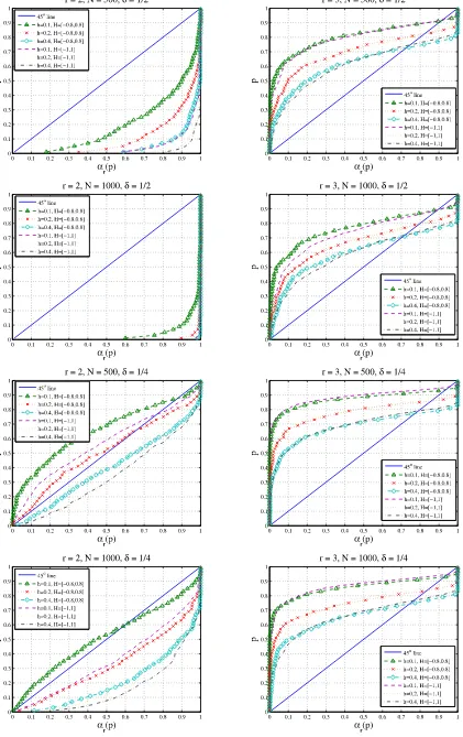
We shall now examine the performance of the global rank tests through a number of PP-plots in Figures2–3. These plots have probabilityp∈(0,1)on the vertical axis againstαr(p)=
P(Tglb(r) >cr(p))on the horizontal axis. Throughout the
sim-ulation study, the probabilityαr(p)is computed based on 500
Monte Carlo replications, andcr(p)is the nominal critical value
such thatP(N(0,1) >cr(p))=p. In kernel smoothing, we use
a popular Epanechnikov kernel, and choose the smoothing para-meterh=0.1, 0.2, or 0.4. IfTglb(r)has the limiting distribution N(0,1), thenαr(p)=p. The caseαr(p) >p[αr(p) <p, resp.]
corresponds toTglb(r)≥dN(0,1)[Tglb(r)≤dN(0,1), resp.].
In Figure2, we provide the PP-plots for various combina-tions of the considered values of the parametersN, δ,h, and
r, and the analysis rangeH. In particular, the PP-plots in the first column correspond to testing for the rankr=2, and those in the second column correspond to testing forr=3. [Testing for r=4 is meaningless since matrices(z)are 4×4. The PP-plots for the cases r=1 and 0 would appear as the cor-responding ones forr=2 with the graphs for the 3 values of
hstretching even more along the bottom-right corner.] Several basic observations can be made at this point. The plots in the second column show that the global rank tests are undersized, even for a large sample size such asN=1000. This is perhaps not surprising in view of our limiting result in Theorem3(ii),
Figure 1. Coordinate functionsfi(x)inf(x)=(fi(x))=(z)V(x)forz= −1/2, 0, and 1. The online version of this figure is in color.
Figure 2. PP-plots in a simulation study. The online version of this figure is in color.
Figure 3. PP-plots in a simulation study. The online version of this figure is in color.
showing thatTglb(r)is asymptotically dominated by (and not
convergent to)N(0,1). Observe also that, as the signal-to-noise ratioδdecreases (more noise), the test is obviously more likely to accept a global rank which is too low. Note also that, when
h decreases, accepting too low a rank is more likely as well. For fixedz, smallerhmeans averaging over fewer data points, leading to a smaller value of a test statistic. Smaller test values overzlead to smaller averaged global test value, leading to a smaller global rank. Finally, the results forH= [−0.8,0.8]and
H= [−1,1]are similar in nature, especially forr=3, suggest-ing that the boundary effects are not that significant. However, this might be due to local rank changes occurring well within the boundary in the model considered.
In terms of size, larger h (oversmoothing) performs better in all plots of Figure 2. Focusing on the first column, over-smoothing also leads to greater power. Though observe that these are not size-adjusted powers. Taking size-adjusting into account would improve the power for smallerh. If the size of test is better when oversmoothing, and the power is better or about the same, we should perhaps use largerhin global rank tests, corresponding to oversmoothing. Note, however, that this may also be the result of our particular model where the local rank changes relatively slowly aszmoves from−1 to 1.
Consider now Figure3where, in the same PP-plots, we com-pare the results forN=500 and 1000. Interestingly, note that the plots for the two sample sizes are close together,
cially forh=0.4. This supports our previous conjecture that the global test statisticTglb(r)has a nonstandard limit
[domi-nated byN(0,1)according to Theorem3(ii)]. As in Figure2, note again how the results are similar forH= [−0.8,0.8]and
H= [−1,1].
In conclusion to this section, we find the simulation results positively surprising. Observe from Figure2that the test does quite well even in the “worst” caseN=500,δ=1/4. Despite intrinsic mathematical proofs, the test therefore seems quite practical, at least for the types of models (6.1)–(6.2) considered here.
7. APPLICATION TO DEMAND SYSTEM
We apply here the introduced global rank test to estimate the global rank of a demand system. See Section1.2for motiva-tion, discussion, and relevant notation. In the dataset used here, budget sharesYiand incomeXi are taken from the U.S. CEX
micro data of the first quarter of 2000. We consider only those households which contain married couples, whose tenure sta-tus is renter household or homeowner with or without mort-gage, whose age of the head is between 25 and 60, and whose total income is between $3000 and $75,000. (We also only consider households in the so-called metropolitan statistical ar-eas because we can associate prices only to these households.) The total number of households which met these criteria was
N=897 (out of 7860 in the CEX dataset). The number of the budget shares considered isj=6. They are expenditures on food, health care, transportation, household, apparel (clothing), and miscellaneous goods.
The pricesZiare drawn from the ACCRA Cost of Living
In-dex dataset (for more information, seehttp:// www.accra.org). ACCRA provides a composite price index and also price in-dices for six different categories of goods for various cities across the U.S. We use throughout only a composite price in-dex and therefore have dim(Zi)=q=1. The pricesZi are
as-signed to(Yi,Xi)by using some location variables in the CEX
dataset as matching variables, and also some confidential in-formation kindly provided by the Bureau of Labor Statistics. (Details on matching procedure are available from the authors upon request.) In the dataset constructed, the values ofZirange
fromzmin=0.911 tozmax=1.251.
We estimate the global rank in the considered demand system as described at the end of Section1.2. First, one budget share is eliminated from the dataset, leading to vectorsYiconsisting of
6−1=5 budget shares. (The test statistic is invariant to which share is eliminated.) Then, the model (1.7) is assumed, where we take
V(x)=
⎛ ⎜ ⎜ ⎝
1 lnx
(lnx)2 (lnx)3
⎞ ⎟ ⎟
⎠. (7.1)
The global rank of the original (full) demand system is esti-mated by adding 1 [see (1.6)] to the estimated global rank of the model (1.7).
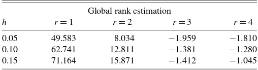
The results of estimation for the original demand system are reported in Table 1. We use the data interval [zmin,zmax] =
[0.911,1.251] for the range of z, and try several values h=
Table 1. Values of test statisticTglb(r)in global rank estimation for a demand system
Global rank estimation
h r=1 r=2 r=3 r=4
0.05 49.583 8.034 −1.959 −1.810 0.10 62.741 12.811 −1.381 −1.280 0.15 71.164 15.871 −1.412 −1.045
0.05, 0.10, and 0.15 for the smoothing parameterh. Note from Table1that the estimated global rank is 3 for all considered val-ues ofh. This perhaps should not be surprising. The same rank can also be found in other work on ranks in demand systems: Lewbel (1991), Donald (1997) where variation in prices is ig-nored, and Fortuna (2008) where local ranks are considered.
Note that Table1above is based on the interval[zmin,zmax] =
[0.911,1.251] spanning the whole range of the values of Zi.
Experimenting with several proper subintervals of[zmin,zmax],
we generally found the global rank to be the same (equal to 3). A potential, interesting exception to the rule, however, seems to be the case of larger values of z. Table2presents global rank estimation results over the interval[1.081,1.251]. Observe that the global rank is estimated as 2 for the smallest considered value ofh.
The statement above is also supported by local rank tests at larger values ofz. For example, Table3gives thep-values for local rank tests atz=1.2. Note that, excepth=0.15, the test points to the local rank 2 atz=1.2. Local rank smaller than 3 for larger values of zwas also found in the same data set but using nonparametric model by Fortuna (2008). To complement Table1, Table4presents thep-values for the local rank test at
z=1. Tests for all the considered values ofhsuggest the local rank 3 atz=1.
APPENDIX A: OUTLINE OF THE PROOF FOR GLOBAL RANK TESTS
Notation and Its Simplification
We suppose for simplicity thatd0=0, that is,(z)=θ(z),
(z)=ψ(z), and similar expressions with the hats. We let Ŵ(z)=−1(z) (z)(z)′be a population version ofŴ(z)in (4.2), and 0≤λ1(z)≤ · · · ≤λm(z)be its ordered eigenvalues.
We shall write
g(z)=θ(z)ψ(z).
Observe that we haveŴ(z)=−1g(z)ψ(z)−1g(z)′and a sim-ilar expression with the hats. To simplify notation further and wherever there is no confusion, we shall drop throughout the
Table 2. Values of test statisticTglb(r)in global rank estimation for a demand system
Global rank estimation
h r=1 r=2 r=3 r=4
0.05 12.724 0.510 −1.406 −1.280 0.10 21.361 4.434 −0.831 −0.905 0.15 30.007 7.214 −0.907 −0.739
Table 3. p-values for local rank test atz=1.2 sponds tom−lzero eigenvalues, and
C′0C0=Im. (A.1)
Similarly, letD0=(D D)be an×nmatrix consisting of the
eigenvectors ofψ−1g′−1gsuch that an×lmatrixD corre-sponds tolnonzero eigenvalues, an×(n−l)matrixD corre-sponds ton−lzero eigenvalues, and
D′0ψD0=In. (A.2)
The next result allows one to replaceλi by the eigenvalues
that are easier to work with asymptotically. The result is stan-dard for fixedz(Robin and Smith2000). See Donald, Fortuna, and Pipiras (2010) for the proof.
Lemma A.1. Under Assumptions1–3,G4–G6, and Table 4. p-values for local rank test atz=1
Local rank estimation atz=1
h r=1 r=2 r=3 r=4
0.05 0 0 0.876 1
0.10 0 0 0.993 1
0.15 0 0 0.994 1
where we used the fact that C′1g=0. The following result is a standard consequence of the Poincaré separation theorem (Magnus and Neudecker1999, p. 209; or Rao1973, p. 65). See Donald, Fortuna, and Pipiras (2010) for the proof.
Lemma A.2. We haveηi≤ξi,i=1, . . . ,m−r.
Define the local and global rank test statistic through the eigenvaluesξiof (A.7) as
Combining LemmasA.1andA.2, we obtain the following re-sult.
Corollary A.1. Under the assumptions of Lemma A.1, we have
The decomposition (A.12) is motivated by the fact that the terms Sj(r) and Sj,glb(r), j =2,4,6, are second-order U
-statistics. We will show (A.11) by arguing thatS1,glb(r)
con-tributes to the asymptotic mean |H|(m−r)(n−r) in (A.9),
S2,glb(r)determines the limiting normal distribution, and the
rest of the termsSj,glb(r),j=3, . . . ,6, are asymptotically
neg-ligible. This is carried out through a number of lemmas below. See Donald, Fortuna, and Pipiras (2010) for the proofs.
Lemma A.3. Under Assumptions1–3,G5–G6, we have LemmasA.1–A.5and CorollaryA.1. Note, in particular, that replacingλibyηiin the global rank statistic using LemmaA.1
requires that(Nhq/ln3N)−1/2h−q/2=(Nh2q/ln3N)−1/2→0, which is one of the assumptions in (5.3). The bias term of the orderO(h2)in (A.14) is negligible when substituted into (A.9) only underq=1,2, or 3, that is, AssumptionG7. Similarly, the terms in (A.17) and (A.18) are negligible whenNhq/2+s
→0 andNhq+2s→0, with the latter convergence implied by the former sincehq+2s=(hq/2+s)2.
Suppose now thatr<supl(z). Then, by smoothness ofθ(z), there is an intervalH0⊂Hsuch thatr<l(z)for all z∈H0.
Then, by using proposition 3.4 in Donald, Fortuna, and Pipiras (2010),
The next elementary result allows one to determine a local rank in a demand system. A bit surprisingly, the result was pre-viously overlooked in the related literature on estimation of ma-trix ranks in demand systems. column eliminated. The second equality in (B.1) holds for any matrixθ(z)where the entries in the first column add up to 1 and those in the other columns add up to 0.
Proof. For notational simplicity, we omit zthroughout the proof. We shall prove the first equality in (B.1). Letr=rk{f(·)} andl=rk{θ}. By the definition of rk{f(·)}, there arej−r ele-ments of a vectorf(x)=θv(x)that can be expressed as linear combinations of the restrelements off(x). Supposing without loss of generality that these are the lastj−relements off(x), combinations of the other r rows. To obtain the converse in-equalityr≤l, observe thatθ=θ1θ2whereθ1is aj×lmatrix
andθ2is al×nmatrix. Then,y=f(x)=θv(x)=θ1(θ2v(x)).
Sinceθ2v(x)is al×1 vector, we obtain from the definition of
local rank thatr≤l. Hence,l=rwhich concludes the first part of the proof.
We will now prove the second equality in (B.1). Setθ= (θ1 θ2)whereθ1 is aj×1 vector andθ2 is aj×(n−1)
matrix. Since the functionsvk(x),k=1, . . . ,n,are linearly
in-dependent andv1(x)=1 by assumption, and since thejbudget
shares add up to 1, we obtain that the elements of the first col-umn of the matrixθadd up to 1 and those in the other columns add up to 0. We want to show first that rk{θ} =rk{θ2} +1.
If the first column of θ can be written as a linear combi-nation of the other columns, that is, for k=1, . . . ,n,θ1k= λ2θ2k+ · · · +λnθnk, λ2, . . . , λn∈R, by summing up all the
equations overk, we get
n is linearly independent of the other columns. This implies that
rk{θ} =rk{θ2} +1. Finally, it is enough to show that rk{θ2} =
rk{}. This holds since the rows ofθ2 add up to 0 and hence
the last row ofθ2is a linear combination of the other rows.
ACKNOWLEDGMENTS
The authors are grateful to Tiemen Woutersen and the par-ticipants of the 2006 North American Winter Meeting of the Econometric Society in Boston for their comments. We would also like to thank the Associate Editor and two referees for many useful suggestions. One of the referees, in particular, has kindly indicated several errors in an earlier version of the arti-cle. CEF.UP—Centre for Economics and Finance at University of Porto—is supported by the Fundação para a Ciência e a Tec-nologia (FCT), Portugal.
[Received November 2007. Revised January 2010.]
REFERENCES
Ahmad, I., Leelahanon, S., and Li, Q. (2005), “Efficient Estimation of a Semi-parametric Partially Linear Varying Coefficient Model,”The Annals of Sta-tistics, 33 (1), 258–283. [295]
Anderson, T. W. (1951), “Estimating Linear Restrictions on Regression Co-efficients for Multivariate Normal Distributions,”Annals of Mathematical Statistics, 22, 327–351. [296,299]
Banks, J., Blundell, R., and Lewbel, A. (1997), “Quadratic Engel Curves and Consumer Demand,”The Review of Economics and Statistics, 79 (4), 527– 539. [296]
Bunse-Gerstner, A., Byers, R., Mehrmann, V., and Nichols, N. K. (1991), “Nu-merical Computation of an Analytic Singular Value Decomposition of a Matrix Valued Function,”Numerische Mathematik, 60 (1), 1–39. [297] Cai, Z., Fan, J., and Li, R. (2000), “Efficient Estimation and Inferences for
Varying-Coefficient Models,”Journal of the American Statistical Associa-tion, 95 (451), 888–902. [295]
Cleveland, W. S., Grosse, E., and Shyu, W. M. (1991), “Local regression mod-els,” inStatistical Models in S, eds. J. M. Chambers and T. J. Hastie, Pacific Grove, CA: Wadsworth/Brooks–Cole, pp. 309–376. [295]
Cragg, J. G., and Donald, S. G. (1993), “Testing Identifiability and Specifica-tion in Instrumental Variable Models,”Econometric Theory, 9 (2), 222–240. [296,298]
(1996), “On the Asymptotic Properties of LDU-Based Tests of the Rank of a Matrix,” Journal of the American Statistical Association, 91 (435), 1301–1309. [296]
(1997), “Inferring the Rank of a Matrix,”Journal of Econometrics, 76 (1–2), 223–250. [296,299]
Donald, S. G. (1997), “Inference Concerning the Number of Factors in a Multivariate Nonparametric Relationship,”Econometrica, 65 (1), 103–131. [299,303]
Donald, S. G., Fortuna, N., and Pipiras, V. (2010), “Technical Appendix for ‘Local and Global Rank Tests for Multivariate Varying-Coefficient Mod-els’,” available at http:// www.fep.up.pt/ docentes/ nfortuna/ jbes_global/ jbes_global_app.pdf. [298,299,304,305]
Fan, J., and Gijbels, I. (1996),Local Polynomial Modelling and Its Applica-tions. Monographs on Statistics and Applied Probability, Vol. 66, London: Chapman & Hall. [296,298]
Fan, J., and Huang, T. (2005), “Profile Likelihood Inferences on Semiparamet-ric Varying-Coefficient Partially Linear Models,”Bernoulli, 11 (6), 1031– 1057. [295]
Fan, J., and Zhang, W. (1999), “Statistical Estimation in Varying Coefficient Models,”The Annals of Statistics, 27 (5), 1491–1518. [295,298]
(2000), “Simultaneous Confidence Bands and Hypothesis Testing in Varying-Coefficient Models,”Scandinavian Journal of Statistics, 27 (4), 715–731. [295]
(2008), “Statistical Methods With Varying Coefficient Models,” Sta-tistics and Its Interface, 1 (1), 179–195. [295]
Fan, J., Zhang, C., and Zhang, J. (2001), “Generalized Likelihood Ratio Sta-tistics and Wilks Phenomenon,”The Annals of Statistics, 29 (1), 153–193. [295]
Fortuna, N. (2008), “Local Rank Tests in a Multivariate Nonparametric Rela-tionship,”Journal of Econometrics, 142 (1), 162–182. [297,303]
Gill, L., and Lewbel, A. (1992), “Testing the Rank and Definiteness of Esti-mated Matrices With Applications to Factor, State-Space and ARMA Mod-els,”Journal of the American Statistical Association, 87 (419), 766–776. [296]
Gorman, W. M. (1981), “Some Engel Curves,” inEssays in the Theory and Measurement of Consumer Behaviour in Honour of Sir Richard Stone, ed. A. Deaton, Cambridge: Cambridge University Press, pp. 7–29. [296] Hastie, T., and Tibshirani, R. (1993), “Varying-Coefficient Models,”Journal of
the Royal Statistical Society, Ser. B, 55 (4), 757–796. [295]
Hausman, J. A., Newey, W. K., and Powell, J. L. (1995), “Nonlinear Errors in Variables: Estimation of Some Engel Curves,”Journal of Econometrics, 65 (1), 205–233. [296]
Karunamuni, R. J., and Alberts, T. (2005), “On Boundary Correction in Kernel Density Estimation,”Statistical Methodology, 2 (3), 191–212. [298] Kato, T. (1976),Perturbation Theory for Linear Operators(2nd ed.).
Grund-lehren der Mathematischen Wissenschaften, Band 132, Berlin: Springer-Verlag. [297]
Kleibergen, F., and Paap, R. (2006), “Generalized Reduced Rank Tests Using the Singular Value Decomposition,”Journal of Econometrics, 133 (1), 97– 126. [296]
Lewbel, A. (1991), “The Rank of Demand Systems: Theory and Nonparametric Estimation,”Econometrica, 59 (3), 711–730. [296,303]
(1997), “Consumer Demand Systems and Household Equivalence Scales,” inHandbook of Applied Econometrics: Microeconomics, Vol. II, eds. M. H. Pesaran and P. Schmidt, Oxford: Blackwell, pp. 167–201. [296] Li, Q., and Racine, J. S. (2007),Nonparametric Econometrics: Theory and
Practice, Princeton, NJ: Princeton University Press. [295,296,298] Li, Q., Huang, C. J., Li, D., and Fu, T.-T. (2002), “Semiparametric Smooth
Coefficient Models,”Journal of Business & Economic Statistics, 20 (3), 412–422. [295,298,299]
Lu, Y. (2008), “Generalized Partially Linear Varying-Coefficient Models,” Journal of Statistical Planning and Inference, 138 (4), 901–914. [295] Magnus, J. R., and Neudecker, H. (1999),Matrix Differential Calculus With
Ap-plications in Statistics and Econometrics(revised ed.), Chichester: Wiley. [304]
Muellbauer, J. (1975), “Aggregation, Income Distribution and Consumer De-mand,”The Review of Economic Studies, 42 (4), 525–543. [296]
(1976), “Community Preferences and the Representative Consumer,” Econometrica, 44 (5), 979–999. [296]
Nicol, C. J. (2001), “The Rank and Model Specification of Demand Systems: An Empirical Analysis Using United States Microdata,”Canadian Journal of Economics, 34 (1), 259–289. [296]
Rao, C. R. (1973), Linear Statistical Inference and Its Applications (2nd ed.).Wiley Series in Probability and Mathematical Statistics, New York– London–Sydney: Wiley. [304]
Robin, J.-M., and Smith, R. J. (1995), “Tests of Rank,” Working Paper 9521, University of Cambridge, Dept. of Applied Economics, Cambridge, U.K. [296]
(2000), “Tests of Rank,”Econometric Theory, 16 (2), 151–175. [299, 304]
Wang, H. (2008), “Rank Reducible Varying Coefficient Model,”Journal of Sta-tistical Planning and Inference, 139 (4), 999–1011. [295]
Xia, Y., Zhang, W., and Tong, H. (2004), “Efficient Estimation for Semivarying-Coefficient Models,”Biometrika, 91 (3), 661–681. [295]