Full Terms & Conditions of access and use can be found at
http://www.tandfonline.com/action/journalInformation?journalCode=ubes20
Download by: [Universitas Maritim Raja Ali Haji] Date: 11 January 2016, At: 22:57
Journal of Business & Economic Statistics
ISSN: 0735-0015 (Print) 1537-2707 (Online) Journal homepage: http://www.tandfonline.com/loi/ubes20
Rank − 1 / 2: A Simple Way to Improve the OLS
Estimation of Tail Exponents
Xavier Gabaix & Rustam Ibragimov
To cite this article: Xavier Gabaix & Rustam Ibragimov (2011) Rank − 1 / 2: A Simple Way to Improve the OLS Estimation of Tail Exponents, Journal of Business & Economic Statistics, 29:1, 24-39, DOI: 10.1198/jbes.2009.06157
To link to this article: http://dx.doi.org/10.1198/jbes.2009.06157
Published online: 01 Jan 2012.
Submit your article to this journal
Article views: 570
View related articles
Rank
−
1/2: A Simple Way to Improve the OLS
Estimation of Tail Exponents
Xavier G
ABAIXDepartment of Finance, Stern School of Business, New York University, 44 West Fourth St., Suite 9-190, New
York, NY 10012-1126 and NBER (xgabaix@stern.nyu.edu)
Rustam I
BRAGIMOVDepartment of Economics, Harvard University, Littauer Center, 1805 Cambridge St., Cambridge, MA 02138 (ribragim@fas.harvard.edu)
Despite the availability of more sophisticated methods, a popular way to estimate a Pareto exponent is still to run an OLS regression: log(Rank)=a−blog(Size), and takebas an estimate of the Pareto exponent. The reason for this popularity is arguably the simplicity and robustness of this method. Unfortunately, this procedure is strongly biased in small samples. We provide a simple practical remedy for this bias, and propose that, if one wants to use an OLS regression, one should use the Rank−1/2, and run log(Rank−
1/2)=a−blog(Size). The shift of 1/2 is optimal, and reduces the bias to a leading order. The standard error on the Pareto exponentζis not the OLS standard error, but is asymptotically(2/n)1/2ζ. Numerical results demonstrate the advantage of the proposed approach over the standard OLS estimation procedures and indicate that it performs well under dependent heavy-tailed processes exhibiting deviations from power laws. The estimation procedures considered are illustrated using an empirical application to Zipf’s law for the United States city size distribution.
KEY WORDS: Bias; Heavy-tailedness; OLS log-log rank-size regression; Power law; Standard errors; Zipf’s law.
1. INTRODUCTION
The last four decades have witnessed rapid expansion of the study of heavy-tailedness phenomena in economics and fi-nance. Following the pioneering work by Mandelbrot (1960, 1963) (see also Fama1965and the papers in Mandelbrot1997), numerous studies have documented that time series encoun-tered in many fields in economics and finance are typically thick-tailed and can be well approximated using distributions with tails exhibiting the power law decline
P(Z>s)∼Cs−ζ, C,s>0, (1.1) with a tail index ζ >0 (see the discussion in ˇCížek, Härdle, and Weron 2005; Rachev, Menn, and Fabozzi2005; Gabaix 2009; Ibragimov 2009, and references therein). Here f(s)∼
g(s) means that f(s)=g(s)(1+o(1)) as s→ ∞. Through-out the paper,Cdenotes a positive constant, not necessarily the same from one place to another. Let
Z(1)≥ · · · ≥Z(n) (1.2) be decreasingly ordered observations from a population satis-fying power law (1.1). Despite the availability of more sophis-ticated methods (see, among others, the reviews in Embrechts, Klüppelberg, and Mikosch1997; Beirlant et al.2004), a pop-ular way to estimate the Pareto exponent ζ is still to run the following OLS log-log rank-size regression withγ=0:
log(t−γ )=a−blogZ(t), (1.3) or, in other words, callingtthe rank of an observation, andZ(t) its size:
log(Rank−γ )=a−blog(Size)
[here and throughout the paper, log(·)stands for the natural logarithm]. WithNdenoting the total number of observations, regression (1.3) with γ =0 is motivated by the approximate linear relationships log(Nt)≈log(C)−ζlog(Z(t)),t=1, . . . ,n, implied by the empirical analogues of relations (1.1). The rea-son for the popularity of the OLS approach to tail index estima-tion is arguably the simplicity and robustness of this method. In various frameworks, the log-log rank-size regressions of form (1.3) in the case γ =0 and closely related procedures were employed, among other works, in Rosen and Resnick (1980), Alperovich (1989), Krugman (1996), Eaton and Eck-stein (1997), Brakman et al. (1999), Dobkins and Ioannides (2000), Davis and Weinstein (2002), Levy (2003), Levy and Levy (2003), Helpman, Melitz, and Yeaple (2004), Soo (2005), and Klass et al. (2006). Further examples and the discussion of the OLS approach to the tail index estimation are provided in Persky (1992), Gabaix et al. (2003, 2009), Eeckhout (2004), Gabaix and Ioannides (2004), and Rossi-Hansberg and Wright (2007).
Letbˆn denote the usual OLS estimator of the tail index ζ using regression (1.3) withγ =0 and let bˆγn denote the OLS estimator ofζ in general regression (1.3).
It is known that the OLS estimatorbˆn in the usual regres-sion (1.3) withγ=0 is consistent forζ. However, the standard OLS procedure has an important bias. This paper shows that the bias is optimally reduced (up to leading order terms) by using
γ=1/2. Therefore, we recommend that, when using a log-log
© 2011American Statistical Association Journal of Business & Economic Statistics January 2011, Vol. 29, No. 1
DOI:10.1198/jbes.2009.06157
24
regression, one should always use log(Rank−1/2)rather than log(Rank).
We further show that the standard error of the OLS estimator
ˆ
bγn of the tail indexζ in general regression (1.3) is asymptoti-cally(2/n)1/2ζ. The OLS standard errors in log-log rank-size regressions (1.3) considerably underestimate the true standard deviation of the OLS tail index estimator. Consequently, taking the OLS estimates of the standard errors at the face value will lead one to reject the true numerical value of the tail index too often.
The 1/2 shift actually comes from more systematic results, in Theorems1and2, which show that it is optimal and further demonstrate that the following asymptotic expansions hold for the general OLS estimatorbˆγn:
E(bˆγn/ζ−1)=(2γ−1)log 2n
4n +o
log2n n
,
ˆ
bγn/ζ =1+
2
nN(0,1)+OP
log2n n
[here and throughout the paper, forμ∈Randσ >0,N(μ, σ2)
stands for a normal random variable (r.v.) with meanμand vari-anceσ2]. We conclude that, when estimating the tail indexζ
with an OLS regression, one should always use the regression log(Rank−1/2)=a−blog(Size),with the standard error of the OLS estimatorbˆnof the slope given by
2
nbˆn.
We further provide similar asymptotic expansions for the tail index estimatordˆnγ in the dual to (1.3) regression
logZ(t)=c−dlog(t−γ ) (1.4) [i.e., log(Size)=c−dlog(Rank−γ )], with logarithms of or-dered sizes regressed on logarithms of shifted ranks. As fol-lows from Theorems 1 and 2, the approaches to the tail in-dex inference using regressions (1.3) and (1.4) are equivalent in terms of the small sample biases and standard errors of the estimators. The paper also discusses asymptotic expansions in the analogues of regressions (1.3) and (1.4) with the logarithms of shifted ranks log(t−γ )replaced by harmonic numbers (Sec-tion3).
Numerical results indicate that the proposed tail index es-timation procedures perform well for heavy-tailed dependent processes exhibiting deviations from power law distributions (1.1) (see Section4). They further demonstrate the advantage of the new approaches over the standard OLS log-log rank-size regressions (1.3) and (1.4) withγ=0.
The tail index estimation methods proposed in the paper are illustrated using an empirical analysis of Zipf’s power law for the United States city size distribution (Section5).
In recent years, several studies have focused on the analy-sis of asymptotic normality of the OLS tail index estimators in regressions (1.4) withγ=0 and logarithms of ordered obser-vations log(Z(t))regressed on logarithms of ranks (see, among other works, the review in chapter 4 in Beirlant et al. 2004). Such an approach to estimation of the tail shape parameters was introduced by Kratz and Resnick (1996) who refer to it as QQ-estimator. Nishiyama, Osada, and Sato (2008) discuss asymptotic normality of the OLS tail index estimator in the re-gression of log(Z(t))on logt. Schultze and Steinebach (1999)
consider closely related problems of least-squares approaches to estimation for data with exponential tails (see also Aban and Meerschaert2004, who discuss efficient OLS estimation of pa-rameters in shifted and scaled exponential models). Kratz and Resnick (1996) establish consistency and asymptotic normal-ity of the QQ-estimator in the case of populations with regu-larly varying tails. Their results demonstrate that in the case of populations in the domain of attraction of power law (1.1), the standard error of the QQ-estimator of the inverse 1/ζ of the tail index based onnlargest observations is asymptotically
√
2/(ζ√n). Csörg˝o and Viharos (1997) prove asymptotic nor-mality of the OLS estimators of the tail index in the caseγ=0 (see also Viharos1999; Csörg˝o and Viharos2006). Beirlant et al. (1999) and Aban and Meerschaert (2004) indicate the possi-bility of modification of the QQ-estimator in which logarithms of ordered observations log(Z(t))are regressed on log(t−1/2). Aban and Meerschaert (2004) mention in a remark without pro-viding a proof that regressing logarithms of observations from a heavy-tailed population on logarithms of their ranks shifted by 1/2 reduces the bias of the QQ-estimator. Their remark seems to be motivated by simulations, not by the systematic under-standing that Theorems1and2provide; in particular, they do not indicate that a shift of 1/2 is the best shift.
To our knowledge, general regressions (1.3) and (1.4) with
γ =0 and asymptotic expansions for them are considered, for the first time, in the present work. The modifications of the OLS log-log rank-size regressions with the optimal shift γ =1/2 and the correct standard errors provided in this paper were sub-sequently used in the works by Hinloopen and van Marrewijk (2006), Bosker et al. (2007), and Gabaix and Landier (2008).
2. FORMAL STATEMENT OF THE RESULTS
Throughout the paper, for variablesa1, . . . ,an,anstands for the sample meanan=1nnt=1at. As usual, for a sequence of r.v.’sXnand a sequence of positive constantsan,we writeXn=
OP(an)[Xn=Oa.s.(an)] if the sequence Xn/an is bounded in probability (resp., bounded a.s.) and writeXn=oP(an)[Xn=
oa.s.(an)] ifXn/an→P0 (resp.Xn/an→a.s.0).
LetZ(1)≥Z(2)≥ · · · ≥Z(n) be the order statistics for a sam-ple from the population with the distribution satisfying the power law
P(Z>s)= 1
sζ, s≥1, ζ >0. (2.1) Denoteyt=log(t−γ )andxt=log(Z(t)). Let us consider the OLS estimatorbˆγn of the slope parameterbin log-log rank-size regression (1.3) withγ <1 and logarithms of ordered observa-tions regressed on logarithms of shifted ranks:
ˆ
bγn= −
n
t=1(xt−xn)(yt−yn)
n
t=1(xt−xn)2 = −
Aγn
Bn
. (2.2)
We will also consider the OLS estimatordˆγn of slope in dual to (1.3) regression (1.4) with logarithms of ordered sizes re-gressed on logarithms of shifted ranks:
ˆ
dγn = −
n
t=1(xt−xn)(yt−yn)
n
t=1(yt−yn)2 = −
Aγn
Dn
. (2.3)
The following theorems provide the main results of the paper.
Theorem 1. For anyγ <1, the following asymptotic expan-sions hold for the bias of the estimatorsbˆγn anddˆγn:
E(bˆγn/ζ−1)= (2γ−1)log 2n
4n +o
log2n n
, (2.4)
E(ζdˆγn−1)= (1−2γ )log 2n
4n +o
log2n n
. (2.5)
Theorem 2. For anyγ <1, the following asymptotic expan-sions hold for the estimatorsbˆγn anddˆγn:
ˆ
bγn/ζ =1+
2
nN(0,1)+OP
log2n n
, (2.6)
ζdˆγn =1+
2
nN(0,1)+OP
log2n n
. (2.7)
The arguments for Theorems1 and2 are presented in the Appendix.
Remark 1. As follows from asymptotic expansions (2.4) and (2.5), the small sample biases of the OLS estimatorsbˆγn anddˆnγ in regressions (1.3) and (1.4) involving logarithms of shifted ranks are both minimized under the choice of the shiftγ=1/2. The proof of Theorems 1 and2 is based on the following results and methods. First, it exploits the Rényi representation theorem to relate the order statistics for observations follow-ing power law (1.1) to the partial sums of scaled iid exponential r.v.’s (see the beginning of the proof of Lemma6). Then, we use martingale approximations to the bilinear forms that appear in the numerators of the statisticsbˆγn/ζ−1= −(Aγn+ζBn)/(ζBn) andζdˆγn−1= −(ζAγn+Dn)/Dn[relation (A.38) in the proof of Lemma6and relation (A.57) in the proof of Lemma8]. Third, the arguments use strong approximations to partial sums of in-dependent r.v.’s provided by Lemma1.
3. A RELATED APPROACH BASED ON
HARMONIC NUMBERS
Fort≥1,denote byH(t)thetth harmonic number:H(t)= t
i=11i. Further, letH(0)=0. Consider the analogues of re-gressions (1.3) and (1.4) that involve logarithms of ordered sizes yt=log(Z(t)) and the functionsx˜t=H(t−1)of ranks of observations:
H(t−1)=a′−b′logZ(t)
, (3.1)
logZ(t)
=c′−d′H(t−1). (3.2) Similar to the proof of Theorem2, one can show that the fol-lowing asymptotic expansions hold for the tail index estimators
ˆ
b′nanddˆ′nusing regressions (3.1) and (3.2):
ˆ
b′n/ζ =1+
2
nN(0,1)+OP
logn
n
, (3.3)
ζdˆ′n=1+
2
nN(0,1)+OP
logn n
. (3.4)
Comparison of expansions (3.3) and (3.4) with (2.4)–(2.7) shows that, ceteris paribus, tail index estimation using regres-sions involving harmonic numbers is to be preferred, in terms of the small sample bias, to that based on the logarithms of
shifted ranks log(t−γ )for anyγ. On the other hand, regres-sions (1.3) and (1.4) are simpler to implement and more visual than estimation procedures based on (3.3) and (3.4). In partic-ular, we are not aware of works that employed estimation ap-proaches based on harmonic numbers similar to (3.3) and (3.4), while regressions (1.3) and (1.4) with γ =0 are commonly used, as discussed in theIntroduction. Comparison of the as-ymptotic expansions for the tail index estimators using regres-sions (3.1) and (3.2) with the OLS tail parameter estimators in log-log rank-size regressions (1.3) and (1.4) also sheds light on the main driving force behind the small sample bias improve-ments using logarithms of shifted ranks log(Rank−1/2). This driving force is, essentially, the fact that log(n−1/2)provides better approximation to the harmonic numbersH(n−1)than does log(n)and, more generally, than log(n−γ ), γ <1. This is because, as follows from the inequalities forH(n)−ln(n+1/2)
in Havil (2003, section 9.3, pp. 75–79), for allγ <1,
H(n−1)=C+ln(n−γ )+(γ−1/2)n−1+O(n−2) (3.5) as n→ ∞, whereC=limn→∞(H(n)−lnn)is Euler’s con-stant, so the optimal choice of the shiftγ in the sense of the best asymptotical approximation is 1/2 [note that the last inequality on p. 76 in Havil2003, should read, in the notations of this sec-tion, 1/(24(n+1)2) <H(n)−ln(n+1/2)−C<1/(24n2)].
4. SIMULATION RESULTS
In this section, we present simulation results on the perfor-mance of the traditional regression (1.3) with γ =0 and the modified regression (1.3) with the optimal shiftγ=1/2 and the correct standard errors given by Theorem2. We present the nu-merical results for the OLS Pareto exponent estimation proce-dures under dependence and under deviations from power laws (1.1). The results are provided for dependent heavy-tailed data that follow AR(1)processesZt=ρZt−1+ut,t≥1,Z0=0,or
MA(1)processesZt=ut+θut−1,t≥1,with iidut’s. The de-partures from power laws are modeled using the innovationsut that have Studenttdistributions with the number of degree of freedomm=2,3,4 (Tables 2and4) or distributions exhibit-ing second-order deviations from Pareto tails in the Hall (1982) form
P(u>s)=s−ζ(1+c(s−αζ−1)), c∈ [0,1), α >0,s≥1,
(4.1)
(Tables1and3). The choice of the number of degrees of free-dom for Studenttdistributions is motivated by the recent em-pirical works on heavy-tailedness that indicate that, for many economic and financial time series, the tail indexζ lies in the interval (2,4) (see Loretan and Phillips 1994; Gabaix et al. 2003, 2009). The benchmark case c=0 in (4.1) corresponds to the exact Pareto distributions (2.1), and the values ρ =0 andθ=0 model iid observationsZt. Similar to deviations of γ from 1/2 in (2.4) and (2.5), the termc(s−αζ −1)modeling the departures from the power laws in (4.1) creates a bias in the estimatorsbˆγn anddˆγn in regressions (1.3) and (1.4).
Tables1 and2 present the simulation results for the tradi-tional OLS estimatorbˆnof the tail index using regression (1.3) withγ =0. These tables also provide the comparisons of the
Table 1. Behavior of the usual OLS estimatorbˆnin the regression log(Rank)=a−blog(Size)for innovations deviating from power laws
Meanbˆn
AR(1) (OLS s.e.) (SDbˆn)
c ρ n 50 100 200 500
0 0 0.924* 0.944* 0.961* 0.978*
(0.024) (0.185) (0.014) (0.134) (0.008) (0.098) (0.004) (0.063)
0 0.5 1.082* 1.069* 1.073* 1.102*
(0.021) (0.296) (0.012) (0.244) (0.007) (0.195) (0.004) (0.145)
0 0.8 1.373* 1.271* 1.235* 1.235*
(0.034) (0.520) (0.019) (0.417) (0.011) (0.343) (0.006) (0.268)
0.5 0 0.925* 0.942* 0.960* 0.978*
(0.024) (0.181) (0.014) (0.132) (0.008) (0.098) (0.004) (0.063)
0.5 0.5 1.082* 1.067* 1.074* 1.104*
(0.020) (0.301) (0.012) (0.244) (0.007) (0.194) (0.004) (0.146)
0.5 0.8 1.379* 1.276* 1.226* 1.238*
(0.034) (0.512) (0.019) (0.412) (0.011) (0.343) (0.006) (0.266)
0.8 0 0.925* 0.945* 0.960* 0.978*
(0.024) (0.186) (0.014) (0.134) (0.008) (0.097) (0.004) (0.063)
0.8 0.5 1.084* 1.067* 1.069* 1.101*
(0.020) (0.297) (0.012) (0.239) (0.007) (0.195) (0.004) (0.145)
0.8 0.8 1.378* 1.270* 1.227* 1.238*
(0.034) (0.520) (0.019) (0.413) (0.011) (0.342) (0.006) (0.265)
MA(1)
c θ
0 0.5 0.988 0.993 1.003 1.032*
(0.024) (0.261) (0.014) (0.193) (0.009) (0.142) (0.004) (0.094)
0 0.8 0.989 0.994 1.011 1.034*
(0.030) (0.275) (0.017) (0.198) (0.010) (0.146) (0.005) (0.098)
0.5 0 0.926* 0.942* 0.961* 0.977*
(0.024) (0.182) (0.014) (0.133) (0.008) (0.099) (0.004) (0.063)
0.5 0.5 0.988 0.992 1.007 1.032*
(0.024) (0.259) (0.014) (0.193) (0.009) (0.142) (0.004) (0.095)
0.5 0.8 0.988 0.992 1.005 1.034*
(0.030) (0.274) (0.017) (0.196) (0.010) (0.145) (0.005) (0.098)
0.8 0 0.925* 0.944* 0.960* 0.978*
(0.024) (0.184) (0.014) (0.134) (0.008) (0.095) (0.004) (0.062)
0.8 0.5 0.991 0.993 1.005 1.030*
(0.024) (0.258) (0.014) (0.192) (0.009) (0.140) (0.004) (0.095)
0.8 0.8 0.990 0.991 1.006 1.033*
(0.030) (0.276) (0.017) (0.198) (0.010) (0.145) (0.005) (0.098)
NOTE: The entries are the estimates of the tail index and their standard errors using regression (1.3) withγ=0 for the AR(1)and MA(1)processesZt=ρZt−1+ut,t≥1,Z0=0, andZt=ut+θut−1,where iidutfollow the distributionP(u>s)=s−ζ(1+c(s−αζ−1)),s≥1,withζ=α=1 andc∈ [0,1). For a general caseζ >0, one multiplies all the numbers in the table byζ. “Meanbˆn” is the sample mean of the estimatesbˆnobtained in simulations, and “SDbˆn” is their sample standard deviation. “OLS s.e.” is the OLS standard error in regression (1.3) withγ=0. The asteric indicates rejection of the true null hypothesisH0:ζ=1 in favor of the alternative hypothesisHa:ζ =1 at the 5% significance level using the reported OLS standard errors. The total number of observationsN=2000. Based on 10,000 replications.
OLS standard errors of the estimator with its true standard de-viation. Tables 3 and 4 present the numerical results on the performance of the OLS estimatorbˆγn using modified regres-sion (1.3) with γ =1/2. In Tables 3 and 4, we also present the standard errors of bˆγn with γ =1/2 provided by expan-sion (2.6) and compare them to the true standard deviation of the estimator. The asterics in Tables1–4 indicate rejection of the true null hypothesis on the tail index H0:ζ =ζ0 in favor
of the alternative hypothesisHa:ζ =ζ0at the 5% significance
level using the reported standard errors [ζ0=1 for innovations
that follow distributions (4.1) with ζ =α=1 considered in Tables1 and3 andζ =mfor innovations that have Studentt
distributions with m=2,3,4 degrees of freedom in Tables2 and4].
For instance, consider the class of exact Pareto iid observa-tions, which is the first row in Tables 1 and 3, with n=50 extreme observations included in estimation. Table1(column
n=50,the first row) shows that the traditional OLS estimator using regression (1.3) with γ =0 yields an average of 0.924 (whereas the true tail index is 1), and the OLS standard error is 0.024, very far from the true standard deviation, 0.185. By con-trast, the OLS estimator using regression (1.3) with γ =1/2 proposed in this paper (Table3, columnn=50,the first row) and expansion (2.6) yield an average estimate of 1.011, and the
Table 2. Behavior of the usual OLS estimatorbˆnin the regression log(Rank)=a−blog(Size)for Studenttinnovations
Meanbˆn
AR(1) (OLS s.e.) (SDbˆn)
m ρ n 50 100 200 500
2 0 1.810* 1.809* 1.768* 1.524*
(0.045) (0.349) (0.026) (0.245) (0.014) (0.160) (0.010) (0.073)
2 0.5 1.993 1.986 1.932* 1.647*
(0.042) (0.454) (0.024) (0.351) (0.014) (0.247) (0.011) (0.115)
2 0.8 2.433* 2.334* 2.199* 1.796*
(0.053) (0.787) (0.031) (0.608) (0.019) (0.429) (0.015) (0.197)
3 0 2.560* 2.503* 2.342* 1.838*
(0.063) (0.473) (0.036) (0.312) (0.021) (0.192) (0.016) (0.079)
3 0.5 2.852* 2.777* 2.597* 1.992*
(0.065) (0.589) (0.037) (0.414) (0.022) (0.262) (0.019) (0.107)
3 0.8 3.632* 3.400* 3.044 2.179*
(0.084) (1.021) (0.049) (0.722) (0.032) (0.448) (0.024) (0.186)
4 0 3.151* 3.002* 2.729* 2.017*
(0.078) (0.546) (0.043) (0.350) (0.027) (0.205) (0.021) (0.083)
4 0.5 3.523* 3.358* 3.024* 2.162*
(0.083) (0.661) (0.047) (0.443) (0.030) (0.259) (0.024) (0.110)
4 0.8 4.546* 4.096 3.516* 2.334*
(0.112) (1.101) (0.065) (0.700) (0.043) (0.417) (0.030) (0.185)
MA(1)
m θ
2 0.5 1.927 1.927* 1.869* 1.602*
(0.044) (0.446) (0.025) (0.325) (0.015) (0.220) (0.011) (0.097)
2 0.8 1.978 1.951 1.894* 1.617*
(0.054) (0.524) (0.031) (0.368) (0.018) (0.242) (0.012) (0.104)
3 0.5 2.774* 2.697* 2.519* 1.944*
(0.064) (0.569) (0.036) (0.400) (0.022) (0.245) (0.018) (0.099)
3 0.8 2.916 2.792* 2.587* 1.974*
(0.075) (0.707) (0.042) (0.464) (0.025) (0.283) (0.019) (0.106)
4 0.5 3.430* 3.253* 2.944* 2.122*
(0.082) (0.649) (0.045) (0.428) (0.029) (0.244) (0.023) (0.099)
4 0.8 3.649* 3.419* 3.035* 2.159*
(0.092) (0.790) (0.052) (0.510) (0.033) (0.287) (0.025) (0.106)
NOTE: The entries are estimates of the tail index and their standard errors using regression (1.3) withγ=0 for the AR(1)and MA(1)processesZt=ρZt−1+ut,t≥1,Z0=0, andZt=ut+θut−1,where iiduthave the Studenttdistribution withmdegrees of freedom. “Meanˆbn” is the sample mean of the estimatesbˆnobtained in simulations, and “SDbˆn” is their sample standard deviation. “OLS s.e.” is the OLS standard error in regression (1.3) withγ=0. The asteric indicates rejection of the true null hypothesis on the tail indexζof ZtH0:ζ=min favor of the alternative hypothesisHa:ζ =mat the 5% significance level using the reported OLS standard errors. The total number of observationsN=2000. Based on 10,000 replications.
standard error of 0.202, very close to the true standard devia-tion, 0.199.
More generally, the OLS estimates bˆn of Pareto exponents ζ using traditional regression (1.3) withγ=0 reported in Ta-bles1and2are significantly different from the true tail indices, which means thatbˆnis biased in small samples. According to the same tables, the OLS standard errors in regression (1.3) with
γ=0 are consistently smaller than the true standard deviations. In most of the numerical results presented in Tables1and2, the true null hypothesis on the tail indexH0:ζ =ζ0 is rejected in
favor of the alternative hypothesisHa:ζ =ζ0at the 5%
signifi-cance level using the OLS standard errors.
In most of the entries in Tables 3 and4, including depen-dence and deviations from power tail distributions, the standard errors in the regression with shiftsγ=1/2 are much closer to the true standard deviations than in the case of the OLS stan-dard errors reported in Tables1and2. Comparing to the
tradi-tional regression in Tables1and2, the approach illustrated by Tables3and4rejects the true null hypothesis on the tail index
H0:ζ =ζ0significantly less often.
Additional simulation results show that regression (1.3) with
γ=1/2 also performs well and dominates the choiceγ=0 for GARCH processes. At the same time, it performs very similar to (3.1) and thus may be preferable due to simplicity.
5. AN EMPIRICAL APPLICATION:
ZIPF’S LAW FOR CITIES
As an example, we study the distribution of city populations (see also Gabaix and Landier2008, where the estimation proce-dures proposed in this paper are used to to confirm a Zipf’s law for market capitalization of large firms). This example is, his-torically, the first economic example of Zipf’s law (Zipf1949), which is the name of power law (1.1) with the tail exponentζ
equal to 1. Zipf’s law is a regularity that has been exerting an
Table 3. Behavior of the OLS estimatorbˆγn withγ=1/2 in the regression log(Rank−1/2)=a−blog(Size) for innovations deviating from power laws
Meanbˆγn=1/2
AR(1) (√2/n×Meanbˆnγ=1/2) (SDbˆγn=1/2)
c ρ n 50 100 200 500
0 0 1.011 1.001 0.998 0.998
(0.202) (0.199) (0.142) (0.139) (0.100) (0.100) (0.063) (0.063)
0 0.5 1.179 1.131 1.112 1.124
(0.236) (0.320) (0.160) (0.257) (0.111) (0.201) (0.071) (0.147)
0 0.8 1.487 1.340 1.277* 1.258*
(0.297) (0.564) (0.189) (0.439) (0.128) (0.354) (0.080) (0.272)
0.5 0 1.013 0.999 0.997 0.998
(0.203) (0.194) (0.141) (0.137) (0.100) (0.101) (0.063) (0.064)
0.5 0.5 1.179 1.129 1.113 1.127
(0.236) (0.326) (0.160) (0.257) (0.111) (0.200) (0.071) (0.147)
0.5 0.8 1.494 1.344 1.268* 1.262*
(0.299) (0.555) (0.190) (0.434) (0.127) (0.354) (0.080) (0.270)
0.8 0 1.013 1.003 0.997 0.998
(0.203) (0.200) (0.142) (0.139) (0.100) (0.099) (0.063) (0.063)
0.8 0.5 1.181 1.129 1.109 1.123
(0.236) (0.322) (0.160) (0.251) (0.111) (0.201) (0.071) (0.147)
0.8 0.8 1.493 1.338 1.269* 1.262*
(0.299) (0.565) (0.189) (0.435) (0.127) (0.353) (0.080) (0.269) MA(1)
c θ
0 0.5 1.078 1.052 1.041 1.053
(0.216) (0.281) (0.149) (0.202) (0.104) (0.146) (0.067) (0.095)
0 0.8 1.078 1.052 1.049 1.054
(0.216) (0.296) (0.149) (0.207) (0.105) (0.149) (0.067) (0.099)
0.5 0 1.014 1.000 0.999 0.998
(0.203) (0.195) (0.141) (0.138) (0.100) (0.101) (0.063) (0.064)
0.5 0.5 1.078 1.051 1.046 1.053
(0.216) (0.279) (0.149) (0.202) (0.105) (0.146) (0.067) (0.096)
0.5 0.8 1.076 1.050 1.043 1.055
(0.215) (0.295) (0.148) (0.205) (0.104) (0.149) (0.067) (0.099)
0.8 0 1.013 1.002 0.998 0.998
(0.203) (0.198) (0.142) (0.140) (0.100) (0.098) (0.063) (0.063)
0.8 0.5 1.081 1.052 1.043 1.051
(0.216) (0.277) (0.149) (0.201) (0.104) (0.144) (0.066) (0.096)
0.8 0.8 1.079 1.049 1.044 1.054
(0.216) (0.297) (0.148) (0.207) (0.104) (0.149) (0.067) (0.099)
NOTE: The entries are estimates of the tail index and their standard errors using regression (1.3) withγ=1/2 for the AR(1)and MA(1)processesZt=ρZt−1+ut,t≥1,Z0=0, andZt=ut+θut−1,where iidutfollow the distributionP(Z>s)=s−ζ(1+c(s−αζ−1)),s≥1,withζ=α=1 andc∈ [0,1). For a general caseζ >0, one multiplies all the numbers in the table byζ. “Meanbˆγ=n 1/2” is the sample mean of the estimatesˆbnγwithγ=1/2 obtained in simulations, and “SDbˆγ=n 1/2” is their sample standard deviation. The values √
2/n×Meanbˆγn=1/2are the standard errors ofbˆγnwithγ=1/2 provided by Theorem2. The asteric indicates rejection of the true null hypothesisH0:ζ=1 in favor of the alternative hypothesisHa:ζ =1 at the 5% significance level using the reported standard errors. The total number of observationsN=2000. Based on 10,000 replications.
enduring interest, because it appears to describe such diverse phenomena as the frequency of words, the popularity of Inter-net sites, the magnitude of earthquakes (see Li2003), and the size of firms (see Axtell2001; Gabaix and Landier2008).
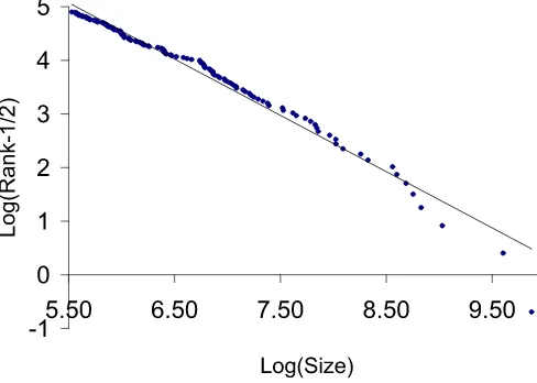
As a U.S. example of a study of Zipf’s law for the cities (in the upper tail at least, see Eeckhout2004), we take, fol-lowing Krugman (1996) and Gabaix (1999), all 135 Ameri-can metropolitan areas listed in the Statistical Abstract of the United States in the year 1991, which includes all agglomera-tions with size above 250,000 inhabitants. The advantage is that “metropolitan area” represents the agglomeration of the cities (e.g., the metropolitan area of Boston includes Cambridge),
which is commonly viewed as the correct economic definition. We rank cities from largest (rank 1) to smallest (rankn=135), and denote their sizesS(1)≥ · · · ≥S(n).
Regression (1.3) withγ=1/2 estimated for the data is log(t−0.5)=10.846−1.050 logS(t).
(0.128)
The number in the bracket is the standard error for the tail in-dex (the slope coefficient bˆγn) given by
2
nbˆn by Theorem 2. Figure1shows the corresponding plot. To plot the correspond-ing log-log graph of the counter-cumulative distribution
Table 4. Behavior of the OLS estimatorbˆγn withγ=1/2 in the regression log(Rank−1/2)=a−blog(Size)for Studenttinnovations
Meanbˆγn=1/2
AR(1) (√2/n×Meanbˆγn=1/2) (True s.e.)
m ρ n 50 100 200 500
2 0 1.981 1.918 1.834 1.552*
(0.396) (0.374) (0.271) (0.255) (0.183) (0.164) (0.098) (0.074)
2 0.5 2.178 2.104 2.004 1.678*
(0.436) (0.489) (0.297) (0.367) (0.200) (0.253) (0.106) (0.116)
2 0.8 2.647 2.465 2.277 1.827
(0.529) (0.854) (0.349) (0.639) (0.228) (0.442) (0.116) (0.200)
3 0 2.798 2.651 2.427* 1.870*
(0.560) (0.507) (0.375) (0.325) (0.243) (0.196) (0.118) (0.080)
3 0.5 3.118 2.941 2.691 2.026*
(0.624) (0.633) (0.416) (0.431) (0.269) (0.268) (0.128) (0.108)
3 0.8 3.956 3.592 3.149 2.215*
(0.791) (1.104) (0.508) (0.756) (0.315) (0.459) (0.140) (0.189)
4 0 3.442 3.177 2.825* 2.051*
(0.688) (0.585) (0.449) (0.364) (0.282) (0.210) (0.130) (0.084)
4 0.5 3.848 3.553 3.130* 2.198*
(0.770) (0.710) (0.502) (0.461) (0.313) (0.265) (0.139) (0.112)
4 0.8 4.950 4.323 3.634 2.370*
(0.990) (1.188) (0.611) (0.732) (0.363) (0.427) (0.150) (0.188) MA(1)
m θ
2 0.5 2.106 2.042 1.939 1.632*
(0.421) (0.480) (0.289) (0.339) (0.194) (0.225) (0.103) (0.098)
2 0.8 2.157 2.065 1.963 1.647*
(0.431) (0.564) (0.292) (0.384) (0.196) (0.248) (0.104) (0.105)
3 0.5 3.032 2.856 2.610 1.978*
(0.606) (0.612) (0.404) (0.417) (0.261) (0.251) (0.125) (0.100)
3 0.8 3.180 2.953 2.679 2.008*
(0.636) (0.761) (0.418) (0.483) (0.268) (0.289) (0.127) (0.107)
4 0.5 3.747 3.441 3.048* 2.157*
(0.749) (0.697) (0.487) (0.446) (0.305) (0.249) (0.136) (0.100)
4 0.8 3.977 3.613 3.140* 2.194*
(0.795) (0.849) (0.511) (0.531) (0.314) (0.293) (0.139) (0.108)
NOTE: The entries are estimates of the tail index and their standard errors using regression (1.3) withγ=1/2 for the AR(1)and MA(1)processesZt=ρZt−1+ut,t≥1,Z0=0, andZt=ut+θut−1,where iiduthave the Studenttdistribution withmdegrees of freedom. For a general caseζ >0, one multiplies all the numbers in the table byζ. “Meanbˆγn=1/2” is the sample mean of the estimatesbˆγnwithγ=1/2 obtained in simulations, and “SDbˆnγ=1/2” is their sample standard deviation. The values√2/n×Meanbˆγn=1/2are the standard errors ofˆbγn withγ=1/2 provided by Theorem2. The asteric indicates rejection of the true null hypothesis on the tail indexζofZtH0:ζ=min favor of the alternative hypothesis Ha:ζ =mat the 5% significance level using the reported standard errors. The total number of observationsN=2000. Based on 10,000 replications.
tion logP(Size>x)vs logxwe recommend to plot log(Size)
on thexaxis, and log((Rank−1/2)/(n−1/2))on theyaxis, rather than the more usual log(Rank/n).
Regression (1.4) withγ=1/2 estimated for the data is logS(t)=10.244−0.930 log(t−0.5),
producing the estimate of the tail index equal to 1/dˆγn ≈1.075 with the standard error given by
2
n
1
ˆ dn ≈0
.131 by Theorem2. The estimates of the tail index are not statistically different from 1 at the 10% significance level, so that Zipf’s law for cities is confirmed in this dataset.
6. CONCLUSION AND SUGGESTIONS
FOR FUTURE RESEARCH
The OLS log-log rank-size regression log(Rank)=a − blog(Size)and related procedures are some of the most
popu-lar approaches to Pareto exponent estimation, withbtaken as an estimate of the tail index. Unfortunately, these procedures are strongly biased in small samples. We provide a simple approach to bias reduction based on the modified log-log rank-size re-gression log(Rank−1/2)=a−blog(Size). The shift of 1/2 is optimal and reduces the bias to a leading order. We further show that the standard error on the Pareto exponentζ in this regres-sion is asymptotically(2/n)1/2ζ,and obtain similar results for the regression log(Size)=c−dlog(Rank−1/2). The proposed estimation procedures are illustrated using an empirical analy-sis of the U.S. city size distribution. Simulation results indicate that the proposed tail index estimation procedures perform well under dependence and deviations from power law distributions. They further demonstrate the advantage of the new methods over the standard OLS log-log rank-size regressions.
An important open problem concerns asymptotic expansions for the OLS tail index estimators and their biases for
Figure 1. Log(Population) vs. Log(Rank− 1/2) for the 135 metropolitan areas in theStatistical Abstract in the U.S., 1991. The slope of the graph corresponds to the estimate of the slope in regres-sion (1.3) with the optimal shiftγ=1/2, and is 1.050 (s.e. 0.128). It is consistent with a Zipf’s law, that is, a power law distribution with the tail index equal to 1. The online version of this figure is in color.
dent processes, including the autocorrelated time series consid-ered in simulations. Combining the modified OLS estimation approach with block-bootstrap and GARCH filters may be use-ful in developing tail index estimation procedures under depen-dence. In addition, unreported preliminary results suggest that the OLS approaches to tail index estimation are more robust than Hill’s estimator of a tail index under deviations from power laws. Other important problems include the analysis of the op-timal choice of the numbern of extreme observations used in estimation and the study of the asymptotic bias of the OLS es-timators whenn is determined by minimizing the asymptotic mean square error. Analysis of these issues and comparisons of the OLS tail index estimators with other procedures are left for further research.
APPENDIX: PROOF OF THEOREMS1AND2
LetZtfollow distribution (2.1), and letZ′t=Z ζ
t. As in (1.2), denote byZ(′1)≥ · · · ≥Z(n)′ decreasingly ordered variablesZt′. We haveP(Zt′>s)=P(Zt>s1/ζ)=1/s,s≥1. Consequently,
Zt′follow distribution (2.1) withζ =1. Evidently, for the loga-rithms of ordered observationsxt=log(Z(t))andx′t=log(Z(t)′ ) one hasxt=x′t/ζ. Therefore, we get that the OLS estimators
ˆ
bγn anddˆnγ in (2.2) and (2.3) satisfy
ˆ
bγn/ζ = − n
t=1(x′t−x′n)(yt−yn)
n
t=1(x′t−x′n)2 ,
ζdˆγn = −
n
t=1(x′t−x′n)(yt−yn)
n
t=1(yt−yn)2 .
This implies that it suffices to prove Theorems1and2for the case ζ =1. This will be assumed throughout the rest of the appendix.
For the proof, we will need the following well-known results provided by Lemmas1–4. Lemma1gives the strong approxi-mation to partial sums of independent r.v.’s that holds under the
assumption of the existence of a moment generating function in a neighborhood of zero. It is provided by, for example, the re-sults in Komlós, Major, and Tusnády (1975) (see also Komlós, Major, and Tusnády1976) and by theorem 2.6.1 on p. 107 in Csörg˝o and Révész (1981).
In Lemma 1, the notation {˜Sn;n =1,2, . . .} =d {Sn;n= 1,2, . . .}means that{Sn}and{˜Sn}are distributionally equiva-lent in the sense that all finite-dimensional distributions of{Sn} and{˜Sn}are the same, that is, the distribution of the random vector(St1, . . . ,Stk)is the same as that of(S˜t1, . . . ,S˜tk)for all
1≤t1<t2<· · ·<tk,k≥1.
Lemma 1. Let Xt,t ≥1, be a sequence of iid r.v.’s with
EXt=0,EXt2=1 such thatR(z)=Eexp(zXt)exists in a neigh-borhood ofz=0. Further, letSn=nt=1Xt,S0=0,stand for
the partial sums ofXt’s. A probability space(,ℑ,P)with a se-quence{˜Sn}and a standard Brownian motionW=(W(s),s≥ 0)on it can be so constructed that{˜Sn;n=1,2, . . .} =d{Sn;n= 1,2, . . .}and|˜Sn−W(n)| =Oa.s.(logn).
Similar to Lemma 1, throughout the rest of the appen-dix,W =(W(s),s≥0)denotes a standard Brownian motion. Lemma 2 concerns the modulus of continuity for Brownian sample paths due to P. Lévy. The asymptotic relation in the lemma is provided, for instance, by theorem 9.25 on p. 114 in Karatzas and Shreve (1991), and by the results in Borodin and Salminen (2002, p. 53).
Lemma 2. The following relation holds:
lim sup δ→+0
1
2δlog(1/δ) 0≤supt1,t2≤1 0<|t2−t1|<δ
|W(t2)−W(t1)| =1 (a.s.).
(A.1)
Lemma3provides an estimate of the rate of growth of sums of independent r.v.’s in terms of their variances. The lemma is a consequence of theorem 6.17 and the discussion following it on p. 222 in Petrov (1995).
In what follows, for a r.v.X withEX2<∞,Var(X)denotes its variance.
Lemma 3. Ifut,t≥1,are independent r.v.’s such thatEu2t <
∞,t≥1, and Vn=Var(nt=1ut)=nt=1Var(ut)→ ∞ as
n→ ∞,thenn
t=1(ut−Eut)=oa.s.(Vn1/2logVn).
Lemma4below is provided by theorem 6.7 in Petrov (1995).
Lemma 4. Letat,t≥1,be positive numbers such thata1≤
a2≤a3≤ · · ·and at→ ∞ as t→ ∞. If ut,t≥1,are inde-pendent r.v.’s such that∞
t=1Var(ut)/a2t <∞,then
n t=1(ut−
Eut)/an→0 a.s. asn→ ∞.
The arguments for the following Lemmas5–9are provided at the end of this appendix. We first formulate, in Lemma 5, several asymptotic relations involving sums of logarithms. De-note
Mn= n−1
t=1
1
t
t
i=1
log(i−γ )−1
n
n
i=1
log(i−γ )
−log(t−γ )+log(n−γ ) 2
, (A.2)
Gn=
Lemma 5. For allγ <1,the following relations hold: n
Relations (2.4) and (2.6) forζ=1 are consequences of (2.2) and the asymptotic expansions for the statisticsAγn andBnunder ζ =1 provided by Lemmas6and7.
Lemma 6. The following asymptotic expansions hold for
ζ =1:
Lemma 7. The following asymptotic relation holds for
ζ =1:
Similar to (2.4) and (2.6), asymptotic expansions (2.5) and (2.7) forζ=1 follow from (2.3) and the asymptotic expansions for the statisticsAγn andDnunderζ =1 provided by Lemmas8 and9.
Lemma 8. The following asymptotic expansions hold for
ζ=1:
Lemma 9. The following asymptotic relation holds for
ζ=1:
Proof of Lemma5. Relations (A.4) and (A.5) follow from Euler–Maclaurin summation formula with the remainder terms that areO(1)for the sums in them (see, e.g., Havil2003, p. 86). Using again Euler–Maclaurin summation formula in a similar way (or first-order integral approximations to partial sums), we obtain (A.6). DenoteLt=1tti=1log(i−γ )−log(t−γ )+1−
Thus, (A.7) indeed holds. From (A.4) we further get
Gn=
This, together with (A.6), implies (A.8). In a similar way, rela-tion (A.9) follows from (A.4), (A.5), and (A.6).
Proof of Lemma6. By the Rényi representation theorem [see Beirlant et al.2004, sections 4.2.1(iii) and 4.4], one has that, for the logarithmsxt=logZ(t)of ordered observations from a population with the distribution satisfying power law (2.1), the transformations
τt=t(xt−xt+1), t=1, . . . ,n−1,
are iid exponential r.v.’s with parameter 1:P(τt>s)=exp(−s),
s≥ 0. That is, one can represent the regressors in (1.3) as weighted sums of exponential r.v.’s in the following way:
xt=xn+zt, t=1, . . . ,n,
We further have
n−1
Using a change of summation indices, we get
n−1
Relations (A.19) and (A.20), together with (A.18), imply
n−1
with the second equality obtained by a change of summation indices similar to (A.19). Using (A.16), (A.21), and (A.22), we get
Similar to the above derivations, we have, using a change of summation indices,
Relations (A.17), (A.24), and (A.25) imply
Aγn=
From (A.23) and (A.26) we get
1
Sinceτt,t≥1,are iid r.v.’s withEτt=1,t≥1,we obtain
Since, by (A.4),
1 from (A.27)–(A.30), it follows that
E(Aγn+Bn)=
whereGnis defined in (A.3). This, together with (A.8), implies (A.10).
Using a change of summation indices, we have that
2
From (A.32) it thus follows that
2
Using this relation, from (A.27) we now obtain
1
where Gn is defined in (A.3). Relations (A.29), (A.30), and Chebyshev’s inequality imply
1
Using relations (A.8) and (A.33)–(A.37), we obtain
1
Let us show that
Un=
one easily obtains that
Qn=O(1). (A.41)
Since, by integral approximations to partial sums [or by (3.5)],
|n−1
that Var(√nUn)=O(1).Thus, (A.39) indeed holds. We now provide the argument for the relation
−√1
using strong approximations to partial sums of independent r.v.’s by Brownian motion.
Using partial summation similar to the proof of lemma 2.3 in Phillips (2007), we get (below,St=ti=1uiandui=τi−1)
By Lemma1, one can expand the probability space as nec-essary to set up a partial sum process that is distributionally equivalent toSt and the standard Brownian motionW(·)on the same space such that
sup
As conventional, throughout the rest of the proof we suppose that that the probability space on which the random sequences considered are defined has been appropriately enlarged so that relation (A.44) holds. From (A.44) we get
n
Let us consider the difference between n
From Lemma2it follows that
sup
In addition, using integration by parts, it is not difficult to see that
From (A.45)–(A.48) and integration by parts it follows that
−√1 (A.42) indeed holds [this relation also follows from (A.45), Lemma2, the relation 1nn
t=1log2(t/n)=2+O( log2n
n ) im-plied by (A.4) and (A.5), and the property that, similar to (A.43), n
Proof of Lemma7. By (A.16), (A.21), and (A.22),
Using (A.50), we also obtain
2
We further have
1
n ). This, together with (A.54), implies that
1
From (A.49), (A.51), (A.53), and (A.55) it follows that (A.12) indeed holds.
From (A.9) and (A.31) it follows that (A.13) indeed holds. Let us show that
Vn=
Similar to the arguments for (A.39), we get that the variance of
Vnsatisfies
Var(√nVn)= n−1
t=1
1
t
t
i=1
log(i−γ )
−
1
n
n
i=1
log(i−γ )
−log(t/n) 2
≤C(Mn+Qn),
whereMnis defined in (A.2) andQnis defined in (A.40). Using (A.7) and (A.41), we thus get that Var(√nVn)=O(1). Conse-quently, (A.58) indeed holds. Relations (A.9), (A.42), (A.57), and (A.58) imply (A.14).
Proof of Lemma 9. Relation (A.15) follows from (A.4), (A.5), and representation (A.56).
ACKNOWLEDGMENTS
We thank the Editor, Serena Ng, an anonymous Associate Editor, two anonymous referees, Gary Chamberlain, Victor Chernozhukov, Graham Elliott, Wolfgang Härdle, Yoko Kon-ishi, Hu McCulloch, Marcelo Moreira, Yoshihiko Nishiyama, Peter Phillips, Artem Prokhorov, Sidney Resnick, Gennady Samorodnitsky, Jim Stock, Jonathan Thong, Charles van Mar-rewijk, Yanping Yi, and the participants at seminars at the De-partments of Economics at Concordia University, Harvard Uni-versity, Institute of Mathematics of Uzbek Academy of Sci-ences, Massachusetts Institute of Technology, Tashkent State University, and Tashkent State University of Economics for helpful comments and suggestions. Gabaix gratefully acknowl-edges support from NSF grant DMS-0527518. Ibragimov grate-fully acknowledges partial research support by the NSF grant SES-0820124, a Harvard Academy Junior Faculty Develop-ment grant and the Clark Fund (DepartDevelop-ment of Economics, Har-vard University).
[Received December 2006. Revised May 2009.]
REFERENCES
Aban, I. B., and Meerschaert, M. M. (2004), “Generalized Least-Squares Es-timators for the Thickness of Heavy Tails,”Journal of Statistical Planning and Inference, 119, 341–352. [25]
Alperovich, G. (1989), “The Distribution of City Size: A Sensitivity Analysis,”
Journal of Urban Economics, 25, 93–102. [24]
Axtell, R. L. (2001), “Zipf Distribution of U.S. Firm Sizes,” Science, 293, 1818–1820. [29]
Beirlant, J., Dierckx, G., Goegebeur, Y., and Matthys, G. (1999), “Tail Index Estimation and an Exponential Regression Model,”Extremes, 2, 177–200. [25]
Beirlant, J., Goegebeur, Y., Segers, J., and Teugels, J. (2004), Statistics of Extremes. Wiley Series in Probability and Statistics, Chichester: Wiley. [24,25,33]
Borodin, A. N., and Salminen, P. (2002),Handbook of Brownian Motion— Facts and Formulae. Probability and Its Applications(2nd ed.), Basel: Birkhäuser. [31]
Bosker, M., Brakman, S., Garretsen, H., de Jong, H., and Schramm, M. (2007), “The Development of Cities in Italy 1300–1861,” Working Paper 1893, CESinfo. [25]
Brakman, S., Garretsen, H., van den Berg, M., and van Marrewijk, C. (1999), “The Return of Zipf: Towards a Further Understanding of the Rank-Size Distribution,”Journal of Regional Science, 39, 182–213. [24]
Csörg˝o, M., and Révész, P. (1981),Strong Approximations in Probability and Statistics, New York: Academic Press. [31]
Csörg˝o, S., and Viharos, L. (1997), “Asymptotic Normality of Least-Squares Estimators of Tail Indices,”Bernoulli, 3, 351–370. [25]
(2006), “Testing for Small Bias of Tail Index Estimators,”Journal of Computational and Applied Mathematics, 186, 232–252. [25]
ˇ
Cížek, P., Härdle, W., and Weron, R. (eds.) (2005),Statistical Tools for Finance and Insurance, Heidelberg: Springer-Verlag. [24]
Davis, D. R., and Weinstein, D. E. (2002), “Bones, Bombs, and Break Points: The Geography of Economic Activity,”American Economic Review, 92, 1269–1289. [24]
Dobkins, L. H., and Ioannides, Y. M. (2000), “Dynamic Evolution of the U.S. City Size Distribution,” inThe Economics of Cities, eds. J. Huriot and J. Thisse, Cambridge: Cambridge University Press, pp. 217–260. [24] Eaton, J., and Eckstein, Z. (1997), “Cities and Growth: Theory and Evidence
From France and Japan,”Regional Science and Urban Economics, 27, 443– 474. [24]
Eeckhout, J. (2004), “Gibrat’s Law for (All) Cities,”American Economic Re-view, 94, 1429–1451. [24,29]
Embrechts, P., Klüppelberg, C., and Mikosch, T. (1997),Modelling Extremal Events for Insurance and Finance, New York: Springer. [24]
Fama, E. (1965), “The Behavior of Stock Market Prices,”Journal of Business, 38, 34–105. [24]
Gabaix, X. (1999), “Zipf’s Law for Cities: An Explanation,”Quarterly Journal of Economics, 114, 739–767. [29]
(2009), “Power Laws in Economics and Finance,”Annual Review of Economics, 1, 255–293. [24]
Gabaix, X., and Ioannides, Y. (2004), “The Evolution of City Size Distribu-tions,” inHandbook of Regional and Urban Economics, Vol. 4, eds. V. Hen-derson and J.-F. Thisse, Amsterdam: Elsevier North-Holland, pp. 2341– 2378. [24]
Gabaix, X., and Landier, A. (2008), “Why Has CEO Pay Increased so Much?”
Quarterly Journal of Economics, 123, 49–100. [25,28,29]
Gabaix, X., Gopikrishnan, P., Plerou, V., and Stanley, H. E. (2003), “A The-ory of Power-Law Distributions in Financial Market Fluctuations,”Nature, 423, 267–270. [24,26]
(2006), “Institutional Investors and Stock Market Volatility,”Quarterly Journal of Economics, 121, 267–270. [24,26]
Hall, P. (1982), “On Some Simple Estimates of an Exponent of Regular Varia-tion,”Journal of the Royal Statistical Society, Ser. B, 44, 37–42. [26] Havil, J. (2003),Gamma: Exploring Euler’s Constant, Princeton, NJ: Princeton
University Press. [26,32]
Helpman, E., Melitz, M. J., and Yeaple, S. R. (2004), “Export versus FDI With Heterogeneous Firms,”American Economic Review, 94, 300–316. [24] Hinloopen, J., and van Marrewijk, C. (2006), “Comparative Advantage, the
Rank-Size Rule, and Zipf’s Law,” Discussion Paper 06-100/1, Tinbergen Institute. [25]
Ibragimov, R. (2009), “Heavy-Tailed Densities,” inThe New Palgrave Dictio-nary Online, eds. S. N. Durlauf and L. E. Blume, Palgrave Macmillan. [24] Karatzas, I., and Shreve, S. E. (1991),Brownian Motion and Stochastic
Calcu-lus, New York: Springer-Verlag. [31]
Klass, O. S., Biham, O., Levy, M., Malcai, O., and Solomon, S. (2006), “The Forbes 400 and the Pareto Wealth Distribution,”Economics Letters, 90, 290–295. [24]
Komlós, J., Major, P., and Tusnády, G. (1975), “An Approximation of Par-tial Sums of Independent RV’s and the Sample DF. I.,”Zeitschrift für Wahrscheinlichkeitstheorie und Verwandte Gebiete, 32, 111–131. [31]
(1976), “An Approximation of Partial Sums of Independent RV’s and the Sample DF. II.,”Zeitschrift für Wahrscheinlichkeitstheorie und Ver-wandte Gebiete, 34, 33–58. [31]
Kratz, M., and Resnick, S. I. (1996), “The QQ-Estimator and Heavy Tails,”
Communications in Statistics. Stochastic Models, 12, 699–724. [25] Krugman, P. (1996),The Self-Organizing Economy, Oxford, U.K. and
Cam-bridge, MA: Blackwell. [24,29]
Levy, M. (2003), “Are Rich People Smarter?”Journal of Economic Theory, 110, 42–64. [24]
Levy, M., and Levy, H. (2003), “Investment Talent and the Pareto Wealth Distri-bution: Theoretical and Experimental Analysis,”Review of Economics and Statistics, 85, 709–725. [24]
Li, W. (2003), “Zipf’s Law Everywhere,”Glottometrics, 5, 14–21. [29] Loretan, M., and Phillips, P. C. B. (1994), “Testing the Covariance Stationarity
of Heavy-Tailed Time Series,”Journal of Empirical Finance, 1, 211–248. [26]
Mandelbrot, B. (1960), “The Pareto–Levy Law and the Distribution of Income,”
International Economic Review, 1, 79–106. [24]
(1963), “The Variation of Certain Speculative Prices,”Journal of Busi-ness, 36, 394–419. [24]
(1997),Fractals and Scaling in Finance. Discontinuity, Concentration, Risk, New York: Springer-Verlag. [24]
Nishiyama, Y., Osada, S., and Sato, Y. (2008), “OLS Estimation and thet
Test Revisited in Rank-Size Rule Regression,”Journal of Regional Science, 48, 691–715. [25]
Persky, J. (1992), “Retrospectives: Pareto Law,”Journal of Economic Perspec-tives, 6, 181–192. [24]
Petrov, V. V. (1995),Limit Theorems of Probability Theory: Sequences of In-dependent Random Variables.Oxford Studies in Probability, Vol. 4, New York: Oxford University Press. [31]
Phillips, P. C. B. (2007), “Regression With Slowly Varying Regressors,” Econo-metric Theory, 23, 557–614. [36]
Rachev, S. T., Menn, C., and Fabozzi, F. J. (2005),Fat-Tailed and Skewed Asset Return Distributions: Implications for Risk Management, Portfolio Selec-tion, and Option Pricing, Hoboken, NJ: Wiley. [24]
Rosen, K. T., and Resnick, M. (1980), “The Size Distribution of Cities: An Examination of the Pareto Law and Primacy,”Journal of Urban Economics, 8, 165–186. [24]
Rossi-Hansberg, E., and Wright, M. L. J. (2007), “Urban Structure and Growth,”Review of Economic Studies, 74, 597–624. [24]
Schultze, J., and Steinebach, J. (1999), “On Least Squares Estimates of an Ex-ponential Tail Coefficient,”Statistcs & Extremes, 2, 177–200. [25] Soo, K. T. (2005), “Zipf’s Law for Cities: A Cross-Country Investigation,”
Re-gional Science and Urban Economics, 35, 239–263. [24]
Viharos, L. (1999), “Weighted Least-Squares Estimators of Tail Indices,” Prob-ability and Mathematical Statistics, 19, 249–265. [25]
Zipf, G. K. (1949),Human Behavior and the Principle of Least Effort, Cam-bridge, MA: Addison-Wesley. [28]