Full Terms & Conditions of access and use can be found at
http://www.tandfonline.com/action/journalInformation?journalCode=ubes20
Download by: [Universitas Maritim Raja Ali Haji] Date: 12 January 2016, At: 17:34
Journal of Business & Economic Statistics
ISSN: 0735-0015 (Print) 1537-2707 (Online) Journal homepage: http://www.tandfonline.com/loi/ubes20
Testing Business Cycle Asymmetries Based
on Autoregressions With a Markov-Switching
Intercept
Malte Knüppel
To cite this article: Malte Knüppel (2009) Testing Business Cycle Asymmetries Based on
Autoregressions With a Markov-Switching Intercept, Journal of Business & Economic Statistics, 27:4, 544-552, DOI: 10.1198/jbes.2009.06117
To link to this article: http://dx.doi.org/10.1198/jbes.2009.06117
Published online: 01 Jan 2012.
Submit your article to this journal
Article views: 52
Testing Business Cycle Asymmetries
Based on Autoregressions With a
Markov-Switching Intercept
Malte K
NÜPPELDeutsche Bundesbank, Wilhelm-Epstein-Straße 14, D-60431 Frankfurt am Main, Germany (malte.knueppel@bundesbank.de)
Implications of two concepts of asymmetry—deepness and steepness—are investigated for autoregres-sive processes with a Markov-switching intercept. The formulas for the skewness of these processes and the skewness of the first differences of these processes are derived. The parameter restrictions leading to nondeepness and nonsteepness are presented for the special case of a first-order autoregression and two states. It is shown that these restrictions imply that previous tests for asymmetries in autoregressive processes with a Markov-switching intercept can lead to wrong conclusions. In an empirical application of the developed tests, the U.S. unemployment rate is found to be steep.
KEY WORDS: Deepness; Regime switching; Skewness; Steepness.
1. INTRODUCTION
Markov-switching models have received much attention in the econometric literature since their first appearance in the seminal article ofHamilton (1989). One of these models’ in-triguing features is their ability to reproduce the asymmetry that is present in many economic time series. In a previous ar-ticle,Clements and Krolzig(2003) developed tests for several asymmetries for models with a Markov-switching mean (here-inafter referred to as MSM models). Two of these asymmetries are deepness and steepness, as defined bySichel(1993).
In this article I extend these tests for deepness and steep-ness to models with a Markov-switching intercept (hereinafter MSI models). MSI models can be appropriate for time series that gradually decrease or increase after a change in regime, whereas MSM models can be used to analyze time series that immediately jump to lower or higher values when a regime change occurs. However, if the persistence within regimes is low, MSI models tend to imply similar behavior as MSM mod-els, so that in this case, the choice between these models is rather arbitrary. Thus MSI models also can be used to, for ex-ample, investigate GDP growth rates, as done byClements and Krolzig(1998), although GDP growth rates tend to be low dur-ing recessions and high durdur-ing expansions, and typically no gradual increase or decrease is observed after a regime change. The tests for deepness and steepness in MSI models require computation of the third moments of these models. These mo-ments are found to depend on the models’ autoregressive pa-rameters. Such a dependency does not apply to MSM models. Therefore, in contrast to what was claimed by Clements and Krolzig(2003), it is not possible to apply tests for deepness and steepness developed for MSM models to MSI models. The con-ditions for nondeepness and nonsteepness in even the simplest MSI processes differ from those in MSM processes. Empirical studies based on MSI processes and Clements and Krolzig’s (2003) tests (as in, e.g., Belaire-Franch and Contreras 2003; Clements and Krolzig 2003; andChen 2005) thus may reach erroneous conclusions.
In an empirical application to the U.S. unemployment rate based on an MSI model setup (Hamilton 2005), I found that
this time series exhibited significant steepness, but no signifi-cant deepness.
This article is organized as follows. Section2briefly presents concepts of asymmetries, and Section3 does so for Markov-switching processes. Section4shows how to test for asymme-tries in MSI models, and also covers the derivation of moments for MSI models. Section5applies the tests for asymmetries to the U.S. unemployment rate, and Section6concludes.
2. CONCEPTS OF ASYMMETRIES
Consider a strictly stationary univariate stochastic process
{Zt}with meanμZ=0 and standard deviationσZ. The process {Zt}is said to be unconditionally symmetric about the mean or,
by convention, shortly symmetric if the marginal distribution of Ztsatisfies
Pr(Zt<−ǫ)=Pr(Zt> ǫ) for allǫ∈R. (1)
Otherwise, the process is said to be asymmetric. To measure the degree of asymmetry, emphasis is placed on the coefficient of skewness ofZt, which is the standardized third central moment,
defined as
τZ=
E[Zt3]
σZ3 . (2)
Following the terminology ofSichel(1993), the type of asym-metry that prevails if τZ <0 is calleddeepness, whereas the
type of asymmetry that prevails ifτZ>0 is calledtallness. Thus
deep distributions are skewed to the left, whereas tall distribu-tions are skewed to the right. IfτZ=0 holds, then the
distribu-tion is said to exhibitnondeepnessor to be not skewed. IfτZ=0
holds but the sign ofτZ is not of interest, I simply speak of the
deepnessofZt. Whether deepness refers toτZ=0 or toτZ<0
is always clear from the context. Nondeepness is a necessary but not sufficient condition for symmetry ofZt.
© 2009American Statistical Association Journal of Business & Economic Statistics
October 2009, Vol. 27, No. 4 DOI:10.1198/jbes.2009.06117
544
Knüppel: Testing Business Cycle Asymmetries 545
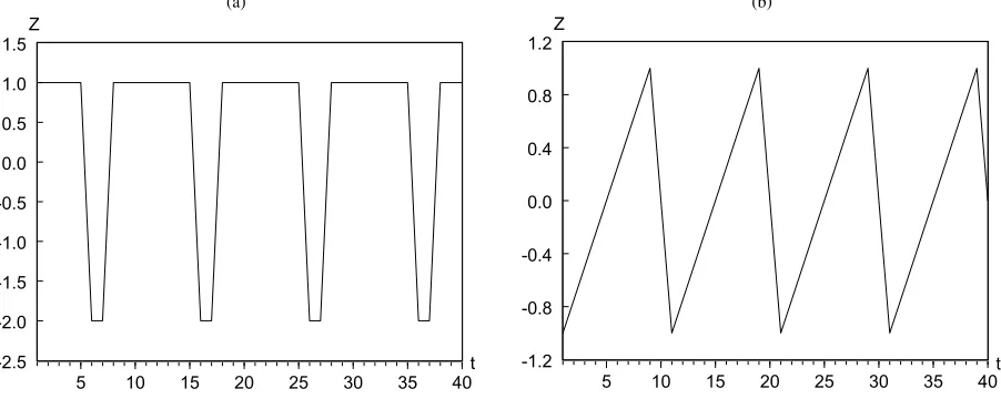
(a) (b)
Figure 1. A deep nonsteep process (a) and nondeep negatively steep process (b).
A related concept of asymmetry deals with the change ofZt
over time, so that the variable of interest is notZt itself, but
rather its first-order differenceZt−Zt−1, denoted byZt. The
stationarity of{Zt}implies μZ =0, whereμZ denotes the
mean ofZt. The standard deviation is denoted byσZ. IfZt
is symmetric, then we have that
Pr(Zt<−ǫ)=Pr(Zt> ǫ) for allǫ∈R (3)
and the degree of asymmetry ofZtagain can be measured by
its coefficient of skewness,
τZ=
E[(Zt)3]
σZ3 . (4)
IfτZ=0 holds, thenZtis said to benonsteep. Otherwise, the
type of asymmetry present inZt is callednegative steepnessif τZ <0 and positive steepnessifτZ>0. Again, this
termi-nology is due mainly toSichel (1993). Exactly as in the case of nondeepness, nonsteepness ofZtis a necessary but not
suffi-cient condition for symmetry ofZt.
Deepness does not imply or prevent steepness, and steep-ness does not imply or prevent deepsteep-ness. These two concepts of asymmetry are mutually independent. To illustrate these con-cepts, Figure1shows examples of a deep but nonsteep process and a negatively steep but nondeep process.
3. MARKOV–SWITCHING PROCESSES
Consider a univariate stochastic process,{st}, wherestadopts
integer valuesiwithi∈ {1,2, . . . ,m}. Suppose further that for this process, Pr(st+1=i|st=j,st−1=k, . . .)equals Pr(st+1= i|st=j)for allt,i, andj. Then the process{st}is said to be an
m-state first-order Markov chain, where the variablest describes
the state (also referred to as regime) of the process in periodt. In what follows, only first-order Markov chains are considered. Allm2transition probabilities,pji=Pr(st+1=i|st=j), are
collected in an(m×m)transition matrixP, defined by
P=
⎡
⎢ ⎢ ⎣
p11 p21 · · · pm1 p12 p22 · · · pm2
..
. ... . .. ... p1m p2m · · · pmm
⎤
⎥ ⎥ ⎦
which is required to be irreducible and to have exactly one eigenvalue on the unit circle. Letγ denote the eigenvector of
Passociated with the unit eigenvalue. For the calculations that follow, it will prove useful to define an(m×1)random vector ξtwhoseith element is equal to unity ifst=iand whose other
elements all equal 0, so that the expectation ofξt+qconditional onξt can be expressed asE[ξt+q|ξt] =Pqξt. Let1mdenote an (m×1)vector of 1’s and normalizeγ so that1′mγ=1. Then it can be shown (cf. Hamilton1994, chap. 22) thatγ contains the unconditional probabilities of each state, so that
γ=E[ξt].
Because the observations of most macroeconomic time se-ries are not realizations of discrete-valued random variables, Markov chains cannot be applied directly to these observa-tions. Instead, the Markov chain must be augmented with a continuous-valued random variable. Commonly, the Markov chain is assumed to govern the state variable of an otherwise standard linear stochastic process with continuous-valued error terms.
The state equation is given by
ξt+1=Pξt+ut+1, (5)
where the zero-mean error vector ut+1 is defined by ut+1= ξt+1−E[ξt+1|ξt]. Given the state equation, a linear
measure-ment equation can be specified by
(L)Zt∗=μ∗st+εt, (6)
where(L)is the lag polynomial(L)=1−ki=1(θiLi),θi
is scalar, andLis the lag operator, so that(1)=1−ki=1θi.
The roots of(L)are required to lie outside the unit circle.Zt∗ shares the properties ofZt except for the zero-mean property.
The error terms {εt}are assumed to be zero-mean
symmetri-cally distributed iid random variables whose variance equalsσε2 and whose third moment exists. The processes of the states{st}
and the error terms{εt}are assumed to be independent. The
in-tercept termμ∗st denotes the value ofμ∗in statest. For instance,
if state two occurs in periodt, thenμ∗st adopts the valueμ∗2in periodt. Thus the process described by (6) contains a Markov-switching intercept and is called a MSI(k)process.
For the calculations that follow, it is convenient to define the vector
μ∗=(μ∗1, μ∗2, μ∗3, . . . , μ∗m)′,
so thatμ∗s t=ξ
′
tμ∗. The elements of the vectorμ∗are required
to have distinct values, so thatμ∗i =μ∗j for alli=j.
For the investigation of central moments, it is useful to write (6) in its mean-adjusted form,
(L)Zt=μst+εt, (7) whereZt=Zt∗−(1)−1γ′μ∗andμst=ξ
′
tμwith
μ=μ∗−1m(γ′μ∗), (8)
so that the variables Zt and μst have the property E[Zt] = E[μst] =0.
As noted byClements and Krolzig(2003), for the study of asymmetry, it is helpful to rewrite (7) as
Zt=(L)−1μst+(L) −1ε
t (9)
that is, as the sum of two independent processes. Because of the symmetry ofεtand its independence of the Markov chain, only
the term (L)−1μst can cause asymmetry of Zt. By the same argument, only the term(L)−1μst can cause asymmetry of Zt=(L)−1μst+(L)
−1ε t.
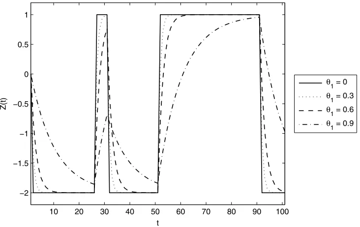
To provide insight into the behavior of MSI(k) processes, consider the plots of MSI(1)processes withθ1=0, θ1=0.3, θ1=0.6, andθ1=0.9 in Figure2. For all of these processes, the number of states equals 2,σε2is set to 0, and all processes follow the same state equation. The vectorμ∗equals [−(1− θ1)2, (1−θ1)1]′.
Three processes gradually approach a certain value after a state change. Only the process withθ1=0 immediately jumps to its new level. It behaves like an MSM process. The value of θ1 determines the speed of approaching a new value ofZt.
A large value ofθ1implies a slow approach.
4. TESTING FOR DEEPNESS AND STEEPNESS IN MSI(k) PROCESSES
As emphasized byClements and Krolzig (2003), asymme-try hypotheses in Markov-switching models can be tested us-ing Wald tests. Testus-ing the null hypothesisf(φ)=0 against the alternativef(φ)=0, whereφ is a vector containing the para-meters of the model andf(φ)is a differentiable function, the well-known Wald test statistic is given by
S=f(φˆ)′ ∂f(φ) ∂φ′
φ= ˆφ
ˆ
∂f(φ) ∂φ′
φ= ˆφ
′−1
f(φˆ), (10)
whereφˆ denotes the maximum likelihood estimator ofφandˆ is its covariance matrix. The functionf(φ)=E[Z3t]/(E[Zt2])3/2 could be used to test the null of nondeepness. Alternatively, the test could be based on the function for the third momentf(φ)=
E[Zt3]. This function and its derivative might be easier to com-pute. Tests of the null of nonsteepness could be conducted by settingf(φ)=E[(Zt)3]/(E[(Zt)2])3/2orf(φ)=E[(Zt)3],
where again it might be easier to use the latter function. Be-causef(φ)is scalar in all cases considered, the test statisticSis asymptoticallyχ2(1)-distributed.
Testing the null hypotheses mentioned earlier requires for-mulas for the third and, depending on the function chosen, pos-sibly also the second moments ofZtandZt.
4.1 Deepness and Steepness of MSI(k) Processes
Concerning the third central moment of MSI(k)processes, to the best of my knowledge, no formula has been docu-mented in the literature. I derive such a formula here. A for-mula for the second central moment of MSI(k)processes was provided by Krolzig (1997, pp. 64–65). But because that for-mula was based on Markov-switching processes in their unre-stricted form, I also present a formula that is more convenient if the Markov-switching process is given in its restricted form.
Figure 2. MSI-processes.
Knüppel: Testing Business Cycle Asymmetries 547
In the restricted form, the elements of the columns ofP, as well as the elements ofγ, sum to 1. In the unrestricted form, this restriction is eliminated.
Proposition 1. The second moment of an MSI(k) process withσε2=0 is given by the first element of the vectorE[Zt⊗
Zt]. This vector can be calculated as
E[Zt⊗Zt]
=(I−⊗)−1
×(e1⊗+⊗e1+(e1⊗e1)μ′Ŵμ), (11)
where the operator⊗denotes the Kronecker product andI de-notes the identity matrix. The(k×1)vectorZtis given by matrix. denotes the vector
=(μ′Ph,μ′P2h, . . . ,μ′Pkh)′, (12)
wherehis given by
h=E[ξtZt] = matrix whose element in rowiand columnjis theith element of the vector ifi=jand 0 otherwise.
Proof. See AppendixA.1.
The second moment ofZtcan be easily calculated using
E[Zt2] =e′1,k2E[Zt⊗Zt] +σ2(L)−1ε, (13) where the unity vectore′
1,k2 is the first column of a(k
2×k2) identity matrix andσ2
(L)−1εdenotes the variance of(L)−1εt.
In what follows,σx2will always denote the variance of the term xt.
Proposition 2. The third moment of an MSI(k) process is given by the first element of the vectorE[Zt⊗Zt⊗Zt]. This
vector can be calculated as
E[Zt⊗Zt⊗Zt]
The matrixQ′is defined by
Q′=E[(Zt⊗Zt)ξ′t]
and can be calculated as
vec(Q′)=(I−P⊗⊗)−1
×vec(e1⊗ + ⊗e1+e1⊗e1(μ2⊙γ)′).
Proof. See AppendixA.1.
Checking for nonsteepness of an MSI(k) process requires considering the equation
Zt=(L)−1μst+(L) −1ε
t. (16)
An investigation of (16) requires the definition of new states related toμst to obtain a first-order Markov chain. This defin-ition implies a new intercept vector,μ, and the corresponding
transition matrix,P. These can be calculated as
μ=μ∗⊗1m−1m⊗μ∗ (17)
and
P=diag(vec(P′))(1m⊗Im⊗1′m). (18)
Appendix A.2 gives an example of such a definition of new states.μ andPcan be inserted into (14), yielding the third
central moment ofZt. If interested in the coefficient of
skew-ness ofZt, then one needs to calculate the variance of Zt.
This can be done by insertingμandP into (11). One also
needs to add the varianceσ2
(L)−1ε.
The deepness of MSI processses can be determined using the formulas (11), (13), and (14). A Wald test for deepness can be conducted by setting f(φ)equal to the first element of (14). Calculating steepness requires (17) and (18) in addition to the three aforementioned formulas. A Wald test for steepness again can be conducted by setting f(φ)equal to the first element of (14), but now usingμandPinstead ofμandP.
It should be noted that the formulas presented for MSI processes also can be used to determine the deepness and steep-ness of MSM processes. In this case, one simply setsk=1 and =θ1=0. The reason for this is that in MSM processes, (9) equalsZt=μst+(L)−
1ε
t, because MSM processes are
char-acterized by(L)(Zt−μst)=εt.
4.2 The Special Case of MSI(1) Processes With Two States
For the special case ofm=2 andk=1, the conditions for nondeepness and nonsteepness can be investigated analytically. This investigation helps highlight the differences between con-ditions for asymmetries in MSI and MSM processes.
Application of (11) shows that the second central moment simplifies to
where θ=θ1. Making use of (14), the third central moment becomes
E[Zt3] =(μ∗2−μ∗1)3(1−p22)(1−p11)(p11−p22)
×((p11+p22−1)2θ3+2(p11+p22−1)
×(θ2+θ )+1)
(1−θ )(2−p11−p22)3
×(θ2+θ+1) 2
i=1
(θi(1−p22−p11)+1) −1
.
(20)
To generate nondeepness for an MSI(1) process with two states, (20) must equal 0. Because we do not consider cases where eitherp11 orp22 equals 1 (this follows from the condi-tions imposed on the transition matrix), it follows that the solu-tions
p11=p22 (21) and
θ2(p11+p22)=θ2−(θ+1)+
(θ2+θ+1) (22)
are feasible. Whereas the nondeepness condition stated in (21) is identical for MSM processes with an arbitrary number of au-toregressive parameters and with two states and identical to the condition for symmetry of two-state MSM and MSI processes, the condition (22) has no counterpart in MSM processes and does not imply symmetry.
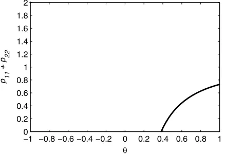
Equation (22) can be illustrated graphically, as done in Fig-ure3. The line represents all combinations ofθ andp11+p22 generating zero deepness whenp11=p22. It is easy to show that combinations on opposite sides of that line give rise to opposite signs of the third central moment if the signs ofμ∗1−μ∗2and p11−p22are identical for these combinations. Thus, in contrast to two-state MSM processes, knowing the signs ofμ∗1−μ∗2and p11−p22is insufficient to determine the sign of the coefficient of skewness of a two-state MSI process.
The investigation of steepness is based on a first-order Markov process forμst. Thus four new states with associated mean vectorμ and transition matrixPmust be defined, as
Figure 3. The thick line depicts all combinations of θ and p11+p22giving rise to nondeepness in two-state MSI(1)-models with p11=p22.
is done in AppendixA.2. The formulas presented for deepness then can be applied to the process forZt. This yields
E[(Zt)2] =(μ∗2−μ∗1)2(2(1−p11)(1−p22))
×(2−p11−p22)(1−(p22+p11−1)θ )
×(θ+1)−1+σ(21−θL)−1ε (23)
and
E[(Zt)3] =(μ∗2−μ∗1)3(3θ (1−p11)(1−p22)(p11−p22))
×
(2−p11−p22)(θ2+θ+1)
×
2
i=1
(θi(1−p22−p11)+1) −1
. (24)
Forp11,p22∈ [0,1), the term (24) equals 0 if
p11=p22 (25)
or
θ=0. (26)
Thus, unlike two-state MSM processes, two-state MSI process-es can exhibit steepnprocess-ess. Consequently, in the case of two statprocess-es, the condition for nonsteepness of MSI(1)processes withθ=0 isalwaysidentical to the condition for nondeepness of MSM processes, not only if |θ| is close to 1, as was claimed by Clements and Krolzig (2003, pp. 202–203).
The example of two-state MSI(1) processes demonstrates that tests for asymmetries developed for MSM processes cannot be directly applied to MSI processes. Suppose that we have an MSI(1)process withθ=0, where condition (22) andp11=p22 hold. Based on the approach ofClements and Krolzig(2003) (i.e., based on the tests for MSM processes), one would con-clude that the MSI(1)process is deep and nonsteep; however, the process actually is nondeep and steep. Table 1 compares all sufficient conditions for deepness and steepness in two-state MSI(1) and MSM processes. The differences between these conditions are linked to the dependency of third-order moments of MSI(1)processes on the autoregressive parameter.
Instead of using the general testing approach for MSI(k) processes described at the end of Section4.1, the null of non-deepness of two-state MSI(1)processes can be tested using the restriction
f(φ)=(p11−p22)
×θ2(p11+p22)−(θ2−(θ+1)+
(θ2+θ+1)),
because this expression equals 0 if (21) or (22) or both equal 0. The restriction for nonsteepness, using (25) and (26), is
f(φ)=(p11−p22)θ.
Knüppel: Testing Business Cycle Asymmetries 549
Table 1. Sufficient conditions for asymmetries in two-state MSI(1) and MSM processes
Sufficient condition(s) for Nondeepness Nonsteepness
in MSI(1)processes p11=p22 p11=p22
θ2(p11+p22)=θ2−(θ+1)+
(θ2+θ+1) θ=0
in MSM processes p11=p22 always nonsteep
5. AN APPLICATION: THE U.S. UNEMPLOYMENT RATE
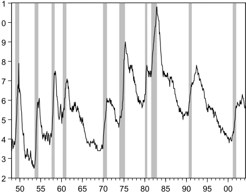
In this section the tests developed earlier are applied to the monthly U.S. unemployment rate from January 1948 to March 2004, using the three-state MSI(2) model setup of Hamilton (2005). As can be seen in Figure4, the unemployment rate typ-ically rises during recessions and falls during expansions. MSI models can reproduce such dynamics because of their regime-dependent intercept term, whereas MSM models clearly are in-appropriate for this time series.
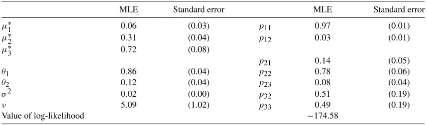
In the Hamilton (2005) model, the error terms are Student t-distributed with scale parameterσ andνdegrees of freedom. The first state of the estimated MSI process corresponds to ex-pansions, the second state corresponds to mild recessions, and the third state corresponds to severe recessions. Motivated by the results of an unrestricted estimation, Hamilton(2005) re-stricted two of the transition probabilities to 0, so that no regime switches occurred from the expansion regime to the severe re-cession regime and vice versa (i.e.,p13=p31=0). Table2 dis-plays the estimation results of the model of Hamilton (2005). Hamilton(2005) found that periods during which the smoothed probabilities of either the second or the third regime attain large values corresponded closely to the recession periods defined by the NBER.
The sample skewness of the U.S. unemployment rate equals τZ =0.52, and its first differences have a sample skewness of τZ=0.31. Thus the U.S. unemployment rate sample exhibits
tallness and positive steepness. The tallness indicates that there were a few periods with an unemployment rate considerably
Figure 4. The U.S. unemployment rate. Shaded areas indicate re-cessions as defined by the NBER.
higher than the average and many periods with an unemploy-ment rate slightly below the average. The positive steepness suggests that the unemployment rate rose very quickly in few periods and decreased slightly in many periods.
I used the restrictions f(φ) = E[Zt3] = 0 and f(φ) =
E[(Zt)3] =0 to evaluate the significance of the
aforemen-tioned asymmetries. To test for deepness, denote the function extracting the first element of (14) byf(φ). Then a Wald test can be performed by calculatingS as in (10). When construct-ing f(φ), bear in mind that μ, not μ∗, must be used so that equation (8) appears inf(φ).
To test for steepness, again denote the function extracting the first element of (14) byf(φ). But in (14),μ andPmust be
used instead ofμandP, so that Equations (17) and (18) appear inf(φ).
Table 3 presents the test results for the null hypotheses of nondeepness and nonsteepness of the U.S. unemployment rate. The derivatives off(φ)are evaluated numerically, because their analytical determination would be very cumbersome.
The null of nondeepness cannot be rejected at conventional significance levels; however, the null of nonsteepness is rejected at the 1% significance level. Thus it can be concluded that the U.S. unemployment rate exhibits significant steepness, imply-ing that the unemployment rate tends to rise more quickly than it falls.
6. SUMMARY
This article has derived formulas for the deepness and steep-ness of MSI processes. Based on these formulas, the tests for deepness and steepness proposed by Clements and Krolzig (2003) for MSM processes can be extended to MSI processes. In contrast to MSM processes, in MSI processes the third mo-ments depend on their autoregressive parameters.
Parameter restrictions for nondeepness and nonsteepness have been presented for the special case of two-state MSI(1) processes. These conditions were shown to be not identical to the corresponding conditions for MSM processes. This re-sult implies that applying tests for asymmetries developed for MSM processes to MSI processes, as suggested byClements and Krolzig(2003), can lead to erroneous conclusions.
The tests for deepness and steepness developed in this ar-ticle have been applied to the U.S. unemployment rate based on a three-state MSI(2)process setup of Hamilton (2005). It turns out that the U.S. unemployment rate is significantly steep, whereas the null of nondeepness cannot be rejected at conven-tional significance levels.
Table 2. Maximum likelihood estimation results of a three-state MSI process for the U.S. unemployment rate
MLE Standard error MLE Standard error
μ∗1 0.06 (0.03) p11 0.97 (0.01)
Value of log-likelihood −174.58
NOTE: MLE, maximum likelihood estimate. Standard errors are computed based on the Hessian.
APPENDIX
A.1 Deepness of MSI Processes
In the calculations that follow, only the regime-switching part of Equation (7) is considered. It is useful to rewrite the measure-ment equation as
Zt=θ1Zt−1+θ2Zt−2+ · · · +θkZt−k+μ′ξt. (A.1)
This equation can be cast in its companion form,
⎡
For the calculations that follow, define a vectorhby
h=E[ξtZt].
Recalling the state equation (5), this definition implies that E[ξt+iZt] =Pih for i=1,2, . . . . With the diagonal matrixŴ
containing the unconditional probabilities of the states on its main diagonal,
Table 3. Wald tests for deepness and steepness of the U.S. unemployment rate
Null hypothesis S p-value
Nondeepness 2.06 0.15
Nonsteepness 6.68 0.01∗
NOTE: The asterisk denotes significance at the 1% level. The covariance matrix is com-puted based on the Hessian.
Second Moments. From (A.2), it follows that the variance ofZtis given by the first element of
E[Zt⊗Zt]
=(⊗)E[Zt−1⊗Zt−1]
+E[vt⊗Zt−1] +E[Zt−1⊗vt] +E[vt⊗vt] (A.3)
Thus, determining the variance ofZtrequires evaluating the last
three terms on the right side of (A.3). Before doing so, it is helpful to define the matrixas in (12). The first term then can be expressed as
On the same lines, the second term is given by
E[Zt−1⊗vt] =⊗e1.
Third Moments. From (A.2), it follows that the third mo-ment ofZtis given by the first element of
E[Zt⊗Zt⊗Zt] =E[Zt−1⊗Zt−1⊗Zt−1]
Knüppel: Testing Business Cycle Asymmetries 551
Thus determining the third moment ofZt requires evaluating
the last seven terms on the right side of (A.4). Start with the first of these terms, which equals
E[vt⊗vt⊗Zt−1]
for the second term and
E[Zt−1⊗vt⊗vt] =E[(μ′ξtξ′tμ)Zt−1] ⊗e1⊗e1
=⊗e1⊗e1
for the third term.
Finding the expressions for the next three terms starts by cal-culating the value ofQ, defined as
Q′=E[(Zt⊗Zt)ξ′t]. be evaluated. The first term equals
E[(vt⊗Zt−1)ξ′t]
where is defined in (A.7). Along the same lines as for the term E[(vt⊗Zt−1)ξ′t], the term E[(Zt−1⊗vt)ξ′t]can be
Finally, solving (A.4) forE[Zt⊗Zt⊗Zt]yields
E[Zt⊗Zt⊗Zt]
=(I−⊗⊗)−1
×e1⊗e1⊗ μ+e1⊗ μ⊗e1
+ μ⊗e1⊗e1+e1⊗(⊗)Q′P′μ
+(⊗)Q′P′μ⊗e1+(⊗e1⊗)Q′P′μ
+(e1⊗e1⊗e1)γ′μ3
.
A.2 A First-Order Markov Process forμst Whenst Has Two States
If st has two states and one is interested in a first-order
Markov process for μst, then one needs to define four new states,
{˜st=1} = {st=1} ∩ {st−1=1},
{˜st=2} = {st=1} ∩ {st−1=2},
{˜st=3} = {st=2} ∩ {st−1=1},
{˜st=4} = {st=2} ∩ {st−1=2},
with associated mean vectorμand transition matrixP.
Cal-culating these according to (17) and (18) gives
μ= ⎡
⎢ ⎣
0 μ1−μ2 μ2−μ1
0 ⎤
⎥
⎦ and
P=
⎡
⎢ ⎣
p11 p11 0 0 0 0 1−p22 1−p22 1−p11 1−p11 0 0
0 0 p22 p22 ⎤
⎥ ⎦.
ACKNOWLEDGMENTS
The author thanks Beatriz Gaitan, James Hamilton, Lothar Knüppel, Wolfgang Lemke, Bernd Lucke, Christian Schu-macher, two anonymous referees, and the editor for very helpful comments and discussions. The author also thanks an anony-mous associate editor for comments that proved to be very valu-able for improving the calculation of moments. Any errors are the author’s. This work represents the author’s personal opin-ion and does not necessarily reflect the views of the Deutsche Bundesbank or its staff.
[Received November 2006. Revised January 2008.]
REFERENCES
Belaire-Franch, J., and Contreras, D. (2003), “An Assessment of International Business Cycle Asymmetries Using Clements and Krolzig’s Parametric Ap-proach,”Studies in Nonlinear Dynamics and Econometrics, 6 (4), Replica-tion 1.
Chen, S.-W. (2005), “Empirical Evidence of Asymmetries in Taiwan’s Business Cycles: A Simple Note,”Taiwan Economic Forecast and Policy, 36 (1), 81– 102.
Clements, M. P., and Krolzig, H.-M. (1998), “A Comparison of the Forecast Performance of Markov-Switching and Threshold Autoregressive Models of US GNP,”Econometrics Journal, 1, C47–C75.
(2003), “Business Cycle Asymmetries: Characterisation and Testing Based on Markov-Switching Autoregressions,”Journal of Business & Eco-nomic Statistics, 21, 196–211.
Hamilton, J. D. (1989), “A New Approach to the Economic Analysis of Nonsta-tionary Time Series and the Business Cycle,”Econometrica, 57, 357–384.
(1994),Time Series Analysis, Princeton, NJ: Princeton University Press.
(2005), “What’s Real About the Business Cycle?”Federal Reserve Bank of St. Louis Review, 87 (4), 435–452.
Krolzig, H.-M. (1997), Markov-Switching Vector Autoregressions, Berlin: Springer.
Sichel, D. E. (1993), “Business Cycle Asymmetry: A Deeper Look,”Economic Inquiry, XXXI, 224–236.