INTEGRATION OF VIDEO IMAGES AND CAD WIREFRAMES
FOR 3D OBJECT LOCALIZATION
R.A. Persad*, C. Armenakis, G. Sohn
Geomatics Engineering, GeoICT Lab Earth and Space Science and Engineering
York University
4700 Keele St., Toronto, Ontario, M3J 1P3 Canada [email protected]
Commission III, WG III/5
KEY WORDS: Image sequences, CAD wireframe, Matching, PTZ camera, Orientation, LR-RANSAC, 3D localization
ABSTRACT:
The tracking of moving objects from single images has received widespread attention in photogrammetric computer vision and considered to be at a state of maturity. This paper presents a model-driven solution for localizing moving objects detected from monocular, rotating and zooming video images in a 3D reference frame. To realize such a system, the recovery of 2D to 3D projection parameters is essential. Automatic estimation of these parameters is critical, particularly for pan-tilt-zoom (PTZ) surveillance cameras where parameters change spontaneously upon camera motion. In this work, an algorithm for automated parameter retrieval is proposed. This is achieved by matching linear features between incoming images from video sequences and simple geometric 3D CAD wireframe models of man-made structures. The feature matching schema uses a hypothesis-verify optimization framework referred to as LR-RANSAC. This novel method improves the computational efficiency of the matching process in comparison to the standard RANSAC robust estimator. To demonstrate the applicability and performance of the method, experiments have been performed on indoor and outdoor image sequences under varying conditions with lighting changes and occlusions. Reliability of the matching algorithm has been analyzed by comparing the automatically determined camera parameters with ground truth (GT). Dependability of the retrieved parameters for 3D localization has also been assessed by comparing the difference between 3D positions of moving image objects estimated using the LR-RANSAC-derived parameters and those computed using GT parameters.
1. INTRODUCTION
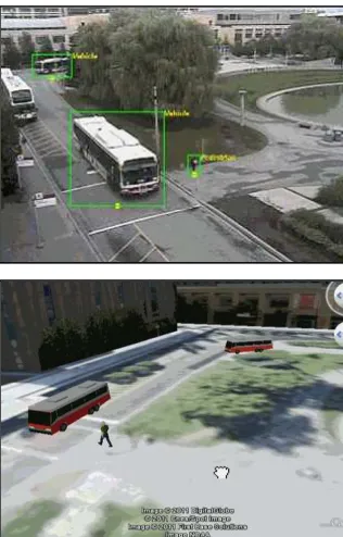
The augmentation and dynamic positioning of 3D moving objects avatars, particularly, vehicles and pedestrians for virtual reality surveillance applications powered by Google Earth and Microsoft Virtual Earth is becoming increasingly important. Figure 1 illustrates the implementation of such a system (Sohn et al., 2011). There has been an extensive amount of work that tries to augment or contextualize 3D virtual environments with dynamic objects from video data (Kim et al., 2009, Baklouti et al., 2009).
Numerous sensors and positioning devices such as GPS, inertial sensors and Radio Frequency IDentification (RFID) are existing technologies which can potentially be used for such purposes. However, these egocentric devices must be attached to the object for tracking and some are impractical for open cityscapes or indoor spaces where for instance, GPS is not functional. Given the widespread use of surveillance cameras, tracking can be performed on a more global basis using video data. The challenge here is the automatic conversion of 2D object positions detected from single images into the 3D space of the reference frame. With the availability of expensive geospatial data sources that have already been used to generate the static 3D building models populating the virtual environment, an approach has been developed which further utilizes this model information for dynamic 3D localization of vehicles and pedestrians.
Figure 1. 3D surveillance prototype. Top: Moving image objects detected from surveillance video. Bottom: 3D visualization of detected objects in Google Earth.
2. OVERVIEW
The transfer of 2D object positions into 3D space requires determination of mapping parameters between camera and the 3D coordinate frames. Traditionally this is done by manually collecting 2D and 3D corresponding features such as points or lines. Then perspective mathematical models are applied to determine the projection parameters. Whenever there is camera motion, this procedure must be repeated. To automate this process, the challenging problem of model-based feature matching (MBFM) must be addressed. MBFM is a coupled problem, i.e. a correspondence and transformation problem. One of these is solvable if the solution to the other is known. Early works in photogrammetry and computer vision have presented several innovative MBFM approaches. Fishler and Bolles (1981) designed the popular RANdom Sample And Consensus (RANSAC) algorithm, Stockman et al. (1982)
proposed the ‘pose clustering’ method, whilst, Grimson and Lozano (1987) developed the ‘interpretation tree’ approach.
Given the current prevalence of geospatial products and data such as airborne LIDAR and digital surface models (DSMs), there has been a recent upsurge in MBFM for various applications. This includes the automated texturing of 3D building models (Wang and Neumann, 2009), and for autonomous robot navigation (Aider et al., 2005). RANSAC-based strategies were used for the mentioned texture mapping works, whilst, Aider et al., (2005) employed the interpretation tree scheme for 2D/3D line matching. In this paper, a MBFM framework utilizing a novel robust estimator called Line-based Randomized RANSAC (LR-RANSAC) is presented. In the first step of the matching process, a common feature matching space must be defined. Automatically detected vanishing points (VPs) are used to determine initial camera parameters enabling the back-projection of model data into image space. To correct errors in the VP-based camera parameters, LR-RANSAC is then applied to obtain an optimal fitting of the model to image. The method utilizes linear segments from both video image data and the geometric 3D wireframes models of man-made structures such as buildings, roads and street furniture vectors for automatic generation of the parameters. Focal length and the 3 image to world rotation angles are considered as the unknown parameters to be estimated (principal point and lens distortions are assumed to be known and zero, respectively) from a Pan-Tilt-Zoom (PTZ) surveillance camera. Camera position is assumed to be rigid and known within the coordinate frame of the 3D model. This is reasonable presumption since surveillance cameras are mounted to a fixed position.
The speed of RANSAC is primarily dependent on a combination of factors such as the number of outliers present in the dataset and the time complexity of the hypothesis verification phase. To minimize the influence of outlying matches, orientation and localization constraints (OLC) and perceptual grouping constraints (PGC) are incorporated in the matching framework. The hypothesis verification scheme used in this work is an evidence search function which proves to be the computational bottleneck of the overall method. To optimize the overall matching time, LR-RANSAC has been implemented and is a modified version of the Randomized RANSAC (R-RANSAC) initially proposed by Chum and Matas (2002). The R-RANSAC algorithm has been described as
‘randomized’ since the decision for executing hypothesis
verification becomes a random process that is subject to the
quality of the random sample set as determined by a ‘pre
-verification’ test. A fast, effective linear feature test has been proposed for LR-RANSAC’s robust estimation framework.
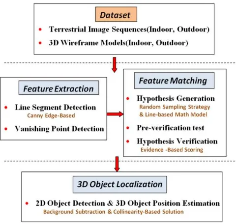
Figure 2. General overview of proposed framework
3. INITIAL REGISTRATION
Outdoor images populated with man-made structures and indoor scenes such as rooms and hallways generally adhere to the Legoland World (LW) assumption. This is an important criterion for the detection of 3 orthogonal VPs. In this work, VPs are used to obtain initial estimates of interior parameters (i.e. focal length), as well as, the camera rotation angles. A sequential-based scoring approach as proposed by Rother (2002) has been employed for estimation of the VPs. Straight line segments are used in the extraction of VPs and are also for the matching phase. The line segments are automatically generated using a Canny edge-based approach (Kovesi, 2011). In the first stage of the registration pipeline, these initial estimates localize the 3D model in image space, where matching can then be performed.
4. OPTIMAL REGISTRATION
There are inherent errors in the VP-based camera parameters. These are due to factors such as image quality and strength of local scene geometry which propagate into the quality of the resulting VP estimates. To refine these parameters, LR-RANSAC is used for matching back-projected wireframe model lines and extracted image lines. LR-RANSAC is an iterative algorithm comprising 3 stages: Hypothesis Generation, Pre-verification Testing and Hypothesis Verification.
4.1 Hypothesis Generation
Constraints. Efficiency of the matching process depends on all possible combinations of model to image matches. The basic premise of any RANSAC-based algorithm is to find a solution in the presence of outliers. Outliers are image lines that erroneously match model lines. To reduce outlying possibilities, PGC and OLC were applied. For PGC, the number of hypothetical matches is lessened by merging broken and multi-detected image line segments that are perceived to be the same. Segments were merged using a least squares fit. Gestalt laws as ISPRS Annals of the Photogrammetry, Remote Sensing and Spatial Information Sciences, Volume I-3, 2012
parallelism and proximity were applied. OLC uses the concept of locally oriented search spaces for random sampling of matches instead of a naive global sampling approach. Similarly oriented image lines were automatically classified into the 3 LW directions as a result of the VP estimation process. Wireframe lines have also been classified a priori according to major LW directions. A significant portion of outliers are removed by limiting the random sampling of model and image lines which belong to the same vanishing direction. One can also assume that the correct image line match for a particular back-projected model line is localized within the vicinity of this model line. Similarly oriented image and model lines are projected into theta-rho (θ-ρ) space. In a similar vein to spatial buffering, the ρ
direction in θ-ρ space is split into buffer-like bins for every
wireframe line in each θ directionand each ρ range. Bin widths are defined empirically for each dataset. Image lines that lie inside these local neighbourhoods are considered as candidate matches for that particular model line.
Cost Function for Matching. Given the randomly sampled correspondence candidates, a camera parameter hypothesis must be established. A line-based mathematical model has been developed for this purpose (Persad et al., 2010). The VP-based parameters are used for initializing the optimization. Refined camera parameters are estimated by adjusting the initial parameters via a minimization of the orthogonal point to line
distance,‘d’, between each pair of corresponding projected model and image lines. Coordinates of the projected model lines, LM are functions of initial camera parameters whereas
those from the image lines, LI are functions of the yet to be defined optimal parameters. The general form of the cost
function, ‘F, used in the non-linear least squares is defined as:
2 outlying matches, the camera parameter hypothesis is considered to be a possible solution. Upon re-backprojecting
the sampled wireframe lines into θ-ρ space, the Euclidean distances between model to image feature points for each randomly sampled model/image line pair should all be reduced or have minimal change compared to their respective distance before the hypothesis had been applied. Reduction in this distance suggests that there is a closer model to image alignment based on the data from this minimal random subset.
Figure 5. Randomly sampled putative matches in θ-ρ space
To confirm, a full verification must be applied globally to the entire dataset. This is dealt with in the next section. If there is
an increase in the distance between wireframe and image θ-ρ feature points after applying the camera parameter hypothesis, the current sample subset is discarded and new ones are generated.
4.3 Hypothesis Verification
The following section describes the process for accumulating the positive and negative evidence using the pre-verified camera parameter hypothesis. All scores are in a normalized 0~1 range.
Positive and Negative Pixel Coverage. Function SC attempts to verify the validity of the hypothesis Hj (where, j is the current LR-RANSAC iteration number)by scoring the ratio of the sum of the overlap of image line pixels PI with the pixels of the
The negative pixel coverage function SN is defined similarly to SC i.e. the ratio of those wireframe pixels not covered by image line pixels to the total number of wireframe pixels. Figure 6 ISPRS Annals of the Photogrammetry, Remote Sensing and Spatial Information Sciences, Volume I-3, 2012
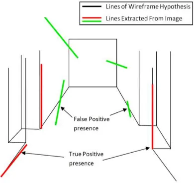
Line Presence. The search for positive line presence is the ratio of extracted image lines that exist over the hypothesized wireframe lines. This differs from the pixel coverage evidence since linear feature characteristics such as orientation and length are taken into account here.
Figure 7. Line presence for Indoor Scene
An image line crossing the model line or in close vicinity to it is considered to be present, however, this can be misleading and the presence support is a false positive as seen in figure 7. In such cases, overlap may be very small and should be classified as a weak line presence. Penalization of false positives has been treated as the modelling of orientation residual error between the model line hypothesis and the candidate image lines that are present on that model line. The modelling of a priori error distribution uses the Laplacian probability density function (pdf). The York Urban Database (Denis et al., 2008), a database of terrestrially captured images comprising of indoor and outdoor man-made scenes, has been used to perform the training for parameter definition in the fitting of this distribution model. From the 102 images in the database, 12 randomly selected images with ground truth (GT) defined lines obtained from manual digitizing were used for training.
Figure 8. Error model for Orientation Residual Scoring
To obtain empirical training data, angular difference between GT lines and automatically established lines are then collected. A GT line and detected line are deemed to be the same line if
they are less than 1.5 pixels apart. Laplace distribution has been used due to the ‘highly peaked’ characteristic and general leptokurtic nature of the empirical data. Figure 8 shows the normalized pdf between 0 and 1. Its estimated fitting parameters were: b=0.66, μ = -0.04. P(∆θ) is the angular residual score. The principal idea of angular residual scoring is to assign a relatively high value if the residual is small. Likewise, if it is high, a low score will be attributed.
,
.
.
(
)
1
m
SF
P
L
L
L
L
SA
m
m
m j
M I I
j M
m
m
(4)Where:
(6)
Weighting by ratio of image to model line length has been used to ensure that presence lines that may be orientation-wise high scoring but possibly only 2 or 3 pixels in length are considered less influential with little significance on the overall scoring. If
|LI| is greater than |LM|, then the weighted length ratio is given a max score of 1. For every model line, a search is performed to determine each image line that intersects it. Each of the image line in the set intersecting the wireframe is individually scored by its angular deviation from the model line, weighted by the ratio of their respective lengths. The summations of the individual scores are then averaged by a fragmentation factor SF, equation 5, which handles multiple broken lines, thus defining a presence score SA for that one particular model line.
SF corresponds to the inverse of the cardinality of the set of line presence candidates m for a single model line. Overall presence score SP, is the ratio of the sum of SA for all model lines to the total number of model lines.
Virtual Corner Presence. The line presence scores propagate into the confidence scores which define the corner support. The 3D corners of the wireframe which are deemed to be present on the image are referred to as virtual corners VC in image space.
Figure 9. Virtual Corner presence for Indoor Scene
e
bb
P
2
1
1
,
2
,
3
...,
m
m
;
m
1
)
m
(
SF
(5)Based on a camera parameter hypothesis for every wireframe corner MCx3D (where, x is the number of corners) defined on the
image, the scores of the individual line presence for two hypothesized wireframe lines forming the VC are averaged into a single score. The total virtual corner presence score, SV is then defined as the ratio of the sum of all the individual VC
presence scores to the cardinality of the set of wireframe corners. SV is defined in equation 7.
VCxFull Verification Score. After the individual scores have been determined from the various evidence knowledge they are combined into a single confidence value to rate Hj. E+ and E- in The hypothesis score SHyp is represented as a linearly weighted
combination of the accumulated evidence. The best fit hypothesis Hyp* is selected according to equation 11, where
Userthres is a user-driven value and N is the max number of set
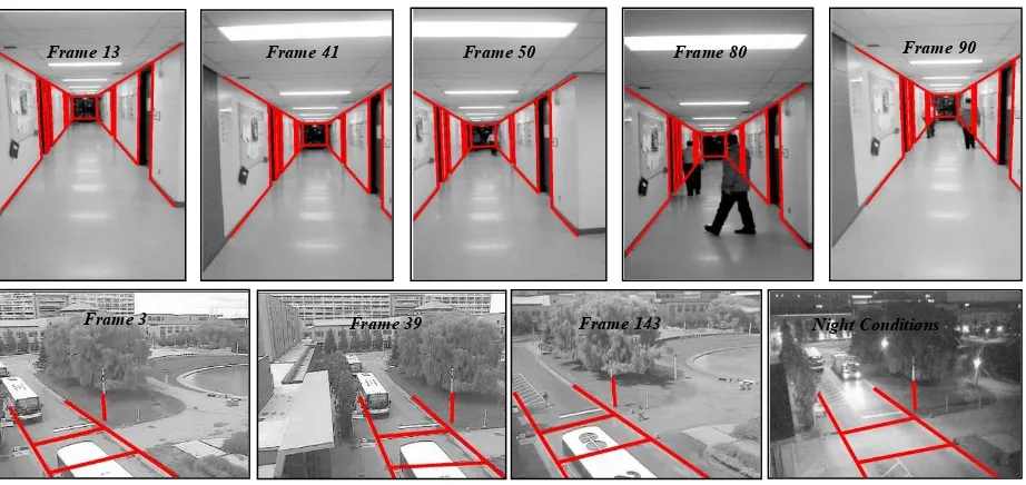
RANSAC iterations (0.8 and 2000 were respective values used for Userthres and N in all experiments). indoor video dataset (94 frames) was taken using a Nikon D90 digital camera mounted onto a tripod with a rotatable panoramic head. The outdoor dataset (144 frames) was obtained using an American Dynamics SpeedDome PTZ camera. Wireframe models have been created using geospatial data such as floor plans, vector data, digital elevation models, orthophotos and LIDAR point clouds. Four line correspondences were used to recover the camera parameters in all experiments. In figure 10, frames 80 and 90 demonstrate the algorithm`s performance in recovering the camera parameters during partial occlusion due to pedestrian movement. The system is also able to match scenes where there is partial occlusion of scene due to camera movement, as shown for frames 41 and 90.
Figure 11. 3D wireframe models used for matching. Indoor model(left).Outdoor road and street post vector(right).
Table 1 show that the uncertainties, σ, are relatively low for all 4 camera parameters
.
For 94 frames of the indoor video sequence, GT camera parameters has been obtained by applying the collinearity equations to 6 pairs of wireframe and image points whose correspondences have been manually defined. The mean absolute errors (i.e., difference between LR-RANSAC and GT parameters) were: 1.6 pixels (0.06mm) for focal length, 0.24º for omega, 0.23º for phi and 0.18º for kappa. In addition to occlusions and aspect changes from camera rotation, the outdoor dataset had movements from frame to frame due to camera zoom coupled with challenging night conditions. Parameter uncertainties were higher in the outdoor dataset. This can be attributed to the lack of well-distributed control geometry on the image during instances where the camera viewing perspective forces the prospective matching to take
Hyp thresFigure 10. Image sequences registered with Wireframe models (red lines). Indoor dataset (Top row). Outdoor dataset (Bottom row).
*
Hyp
Frame 13 Frame 41 Frame 50 Frame 80 Frame 90
Frame 3 Frame 39 Frame 143 Night Conditions
Table 1. LR-RANSAC derived camera parameters across several frames from indoor and outdoor image sequences
place in a small concentrated section of the image space. It is
assumed that the lack of matching features in these ‘control free’ image areas increases the level of uncertainty in estimated
parameters. Based on GT comparison across 144 frames, mean absolute errors for parameters were: 13.2 pixels (0.07mm) for focal length, 0.28º for omega, 0.19º for phi and 0.30º for kappa. Based on general angular errors, accuracies are in the order of 1/285 and 1/200 for the indoor and outdoor dataset respectively.
Tests were also done for 3D object localization. For this experiment, two static image sequences in the indoor and outdoor test areas were used. Background subtraction was used to detect a single moving object in each area, i.e. pedestrian for indoor and vehicle for outdoor. The 2D detected object locations are only an approximate indication of the true ground position (i.e. the base of the fitted image-based bounding box). Inverse collinearity was used to estimate planimetric (X and Y) model positions of each detected object, with the ground plane Z coordinate constrained to zero. To quantify accuracies of the object positions in the 3D model, the difference in positions estimated using automatically determined camera parameters from those estimated with GT are considered to be errors. In the outdoor dataset, the mean X and Y error for objects within 50m from the camera is 0.2m and 0.65m respectively. In the indoor dataset, the mean X and Y error for objects within 10m from the camera is 0.006m and 0.3m respectively.
6. CONCLUSIONS
A framework which automatically matches 3D wireframe models to images for dynamic camera parameter retrieval has been presented. Results show that the estimation of camera parameters for model-space localization is within tolerable accuracies. Registration takes 12 seconds on average per frame with un-optimized MATLAB code (line extraction and vanishing point processes take a combined 7 seconds (bottleneck of overall algorithm) and LR-RANSAC takes 4 seconds). Real time efficiency is expected and future work will address such limitations with conversion to a low level language and use of parallel processing. With these minor improvements, practical use for object localization in virtual reality-based surveillance applications would be seamless.
ACKNOWLEDGEMENTS
This work was financially supported by the Natural Sciences and Engineering Research Council of Canada (NSERC) and the Geomatics for Informed Decisions (GEOIDE) network.
REFERENCES
Aider, O.A , Hoppenot, P. and Colle, E. (2005). A model-based method for indoor mobile robot localization using monocular vision and straight-line correspondences. Robotics and Autonomous Systems, 52, pp. 229-246.
Baklouti, M., Chamfrault, M., Boufarguine, M. and Guitteny, V. (2009). Virtu4D : A dynamic audio-video virtual representation for surveillance systems . 3rd International Conference on Signals Circuits and Systems, v. 6-8, pp. 1-6 .
Chum, O. and Matas, J. (2002). “Randomized RANSAC with
td,d test”. In P. Rosin and D. Marshall, (Eds.), Proceedings of the British Machine Vision Conference, Volume 2, pages 448-457.
Denis, P., Elder, J., and Estrada, F. (2008).Efficient edge-based methods for estimating Manhattan frames in urban imagery. In Proceedings of Euro. Conf. Comput. Vision, pp. 197–210
Fischler, M., and Bolles, R. (1981). Random sample consensus: a paradigm for model fitting with applications to image analysis and automated cartography. Comm. ACM, 24(6).
Grimson, W. E. L. and Lozano-Perez, T. (1987).Localizing Overlapping Parts by Searching the Interpretation Tree. IEEE Transactions on Pattern Analysis and Machine Intelligence, 9(4), pp.469-481.
Kim, K., Oh, S., Lee J., and Essa, I. (2009). Augmenting Aerial Earth Maps with Dynamic Information. IEEE International Symposium on Mixed and Augmented Reality 2009, Science and Technology Proceedings, pp. 19–22.
Kovesi, P. D. (2011). MATLAB and Octave functions for computer vision and image processing. Centre for Exploration Targeting, School of Earth and Environment, The University of Western Australia.
Persad, R.A., Armenakis, C. and Sohn, G. (2010). Calibration of a PTZ Surveillance Camera using 3D Indoor Model.
Proceedings of Canadian Geomatics Conference 2010 and ISPRS Com 1 Symposium, Calgary, International Archives of the Photogrammetry, Remote Sensing and Spatial Information Sciences, Vol.XXXVIII Part 1.
Rother, C. (2002). A new approach to vanishing point detection in architectural environments. Image Vis. Comput., 20(9– 10):647 – 655.
Sohn, G., Wang, L., Persad, R.A., Chan, S., and Armenakis, C. (2011). Towards dynamic virtual 3D world: Bringing dynamics into integrated 3D indoor and outdoor virtual world. The Chinese Academic Journal. Joint ISPRS workshop on 3D City Modeling and Applications and the 6th 3D GeoInfo, Wuhan, China.
Stockman, G., Kopstein, S., and Benett, S. (1982). Matching Images to Models for Registration and Object Detection via Clustering. IEEE Transactions on Pattern Analysis and Machine Intelligence, vol. 4 , no. 3, pp.229-241.
Wang, L., Neumann, U. (2009). A robust approach for automatic registration of aerial images with untextured aerial LIDAR data. In: Proc. of CVPR.
Frame fpix ± (σpix) ωº± (σ") φº± (σ") κº± (σ") Indoor dataset
13 541 ± 1.6 -9.9 ± 4.7 -1.2 ± 2.9 -1.1 ± 4.3
41 542 ± 0.2 -3.5 ± 0.4 -3.2 ± 0.4 -0.8 ± 1.1
50 544 ± 6.0 -2.9 ± 40 -4.9 ± 33 -1.4 ± 34
80 540 ± 5.9 -0.7 ± 21 -0.9 ± 15 -1.1 ± 36
90 527 ± 3.1 -9.9 ± 8.3 3.8 ± 5.8 -0.5 ± 18
Outdoor dataset
3 667 ± 6.2 -12 ± 39 -30 ± 37 -4.9 ± 79
39 716 ± 5.2 -12 ± 35 -11 ± 32 -0.7 ± 111
143 724 ± 5.5 -16 ± 25 -30 ± 20 -7.3 ± 62
Night Cond. 722 ± 3.9 -15 ± 14 -22 ± 17 -5.4 ± 45