Saving Behavior
Libertad González
Berkay Özcan
A B S T R A C T
We analyze the causal impact of an increase in the risk of marital dissolution on the saving behavior of married couples. We use the legalization of divorce in Ireland in 1996 as an exogenous shock to the risk of divorce. We propose several comparison groups (unaffected by the law change) that allow us to use a difference- in- differences approach. Our fi ndings suggest that the legalization of divorce led to a signifi cant increase in the propensity to save by married individuals, which is consistent with individuals saving more as a response to the increase in the probability of marital breakup.
I. Introduction
This paper aims to test empirically the causal effect of an increase in marital instability on the saving behavior of married individuals. Previous theoretical studies have not been able to unambiguously sign this effect, due to confl icting chan-nels at work. We use the legalization of divorce in Ireland in 1996 as an exogenous shock to the risk of divorce. We propose several comparison groups (unaffected by the law change) that allow us to follow a difference- in- differences approach. Our fi ndings suggest that the legalization of divorce led to a sizeable increase in the propensity to save by married individuals.
The authors are listed alphabetically and have contributed equally. Libertad González is an associate pro-fessor at Universitat Pompeu Fabra and an affi liated professor at the Barcelona GSE. Berkay Özcan is an assistant professor (lecturer) at the London School of Economics and Political Science. They are grateful to Justin Wolfers, Ernesto Villanueva, Gosta Esping- Andersen, Douglas McKee, Climent Quintana- Domeque and Juho Härkönen for comments that improved earlier versions of the paper. They also thank seminar participants at the University of Essex, Universitat Pompeu Fabra, University College Dublin and Stony Brook University, and attendees at the IFN Stockholm Conference on Family, Children and Work and the III Workshop on the Economics of the Family at the University of Zaragoza. Financial support from the Spanish government (ECO2011-25272) is gratefully acknowledged. The data used in this article can be obtained beginning October 2013 through September 2016 from Libertad González, Universitat Pompeu Fabra, Department of Economics and Business, Ramon Trias Fargas 25-27, 08005, Barcelona / Spain. E- mail: libertad.gonzalez@upf.edu
[Submitted May 2011; accepted May 2012]
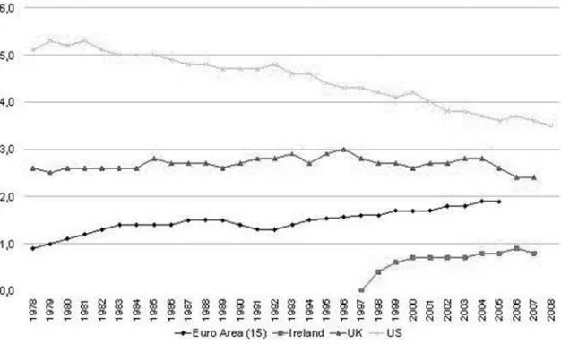
Marital instability has been high for several decades in most OECD countries, al-though with large variation across geographical regions and demographic character-istics. For example, the divorce rate in the United States has been traditionally high by international standards, reaching more than fi ve divorces per 1,000 people around 1980, and declining ever since to current rates below four (see Figure 1). In stark contrast, there was only about one divorce per 1,000 people in the EU- 15 in 1980, up to almost two in 2005.
Economists and demographers have long been interested in understanding how the risk of marital breakdown affects individual behavior and well- being. The most com-mon outcome of interest has probably been labor supply, especially of the female spouse (Johnson and Skinner 1986; Parkman 1992; Papps 2006; Stevenson 2008). Other outcomes that have received some attention are the degree of specialization within the marriage (Lundberg and Rose 1999), the division of labor between the spouses (Lommerund 1989), and the investment in marriage- specifi c capital (Steven-son 2007). The fi ndings to date suggest that an increase in the risk of divorce may lead to increases in labor supply (especially among women) and a decline in marriage- specifi c investments. The saving behavior of households, although a relevant outcome that can potentially be affected by the risk of divorce, has not been investigated em-pirically to our knowledge.
A popular empirical strategy in the most recent studies is to exploit the variation across U.S. states in the introduction of unilateral divorce legislation.1 However, re-cent research suggests that the effect of unilateral legislation on divorce rates may
1. “Unilateral divorce” laws allow people to get a divorce without the consent of their spouse. Figure 1
have been limited in the long term (Wolfers 2006), which raises the question of how much unilateral divorce effectively affected the perceived risk of marital separation. At the same time, European countries have in recent decades undergone much broader reforms in their divorce legislation, and some countries have even legalized divorce fairly recently, such as Spain in 1981 or Ireland in 1996, resulting in signifi cant in-creases in divorce rates (González and Viitanen 2009). We thus exploit the recent legalization of divorce in Ireland in the view that it provides a stronger shock to the risk of divorce than the legal reforms previously exploited in the literature.
The determinants of the saving behavior of individuals and households has long been the subject of study by economists, but we are still far from reaching full under-standing of the factors that drive consumption and saving decisions.2 The standard stylized models of saving do not account explicitly for life- changing events such as marriage and divorce, which have potentially relevant and long- lasting implications for income and consumption.3 This is regrettable given the high levels of marital in-stability reached in many OECD countries, which may well have had a signifi cant impact on saving rates.
Some recent theoretical work has made an attempt to introduce marriage and di-vorce explicitly in a model of savings,4 stressing different channels through which marital transitions can affect consumption and savings. They do not, however, provide an unambiguous prediction regarding the effect of increasing marital instability on the saving behaviour of married couples.
Divorce is generally viewed as a costly event (lawyer fees, etc). Moreover, the economies of scale associated with marriage are lost upon marital dissolution. There-fore, a rise in the perceived risk of divorce would be viewed by the married individual as an increase in the probability of experiencing a negative shock. This is in turn expected to lead to higher precautionary savings, similar to the effect of an increase in labor income risk (Cubbedu and Ríos- Rull 1997).
However, a divorce also implies that the common assets of the couple must be split between the partners. Thus, an increase in the likelihood of divorce would make saving while married more risky, creating incentives to increase current consumption (Mazzocco et al. 2007).
There are additional channels that also can lead to a negative relationship between the risk of marital instability and savings—for instance, if divorce involves fees that reduce the net worth and thus the return to saving of the couple, or if divorce is po-tentially followed by remarriage, which implies that individual assets will have to be shared with the new partner (Cubbedu and Ríos- Rull 1997).
Overall, the expected effect of an increase in the risk of divorce on the saving be-havior of the spouses is ambiguous, thus the need for empirical work to test which of the channels dominates in practice. To our knowledge, we provide the fi rst empirical test for the effect of the increase in the risk of marital instability on the saving behavior of married couples. In order to do so, we take advantage of an exogenous increase
2. An example is the lack of consensus in the literature regarding the source of the drastic fall in saving rates in the United States since the 1980s (Browning and Lusardi 1996).
3. There are some exceptions, such as Browning (2002), who models the saving behavior of married couples, and Browning et al. (2009), who address the impact of marriage on consumption and saving.
in the risk of marital dissolution generated by the recent legalization of divorce in Ireland, and follow a difference- in- differences approach to identify its effect on house-holds’ propensity to save.
Using individual- level, longitudinal data, we fi nd that married couples in Ireland saved more after 1996, both in absolute terms and relative to single individuals and to married couples in other European countries. Moreover, the increase was particularly pronounced for nonreligious marriages, relative to religious ones.
Our main result, that married couples affected by the legalization of divorce in-creased their savings after the reform, is consistent when using three different control groups and across three independent data sets and eight different measures of saving behavior, and does not seem to be driven by the overall improvement in economic conditions. We interpret the evidence as consistent with an increase in saving by mar-ried individuals in response to the increase in the risk of divorce.
The remainder of the paper is organized as follows. Section II introduces the data and the methodology. First we provide support for our identifying assumption that the Irish divorce law of 1996 led to an increase in the risk of marital dissolution. We then propose several alternative control groups (religious Irish couples, Irish singles, married couples in other European countries) and provide support for the claim that, while they were subject to similar economic conditions, they did not experience an increase in the risk of divorce as a result of the law change. Next we introduce the econometric specifi cation and we discuss the measures of saving behavior available in the data. Section III discusses the results when using the alternative control groups, and Section IV concludes.
II. Data and Methodology
A. The Irish Divorce Law
We propose to identify the effect of an increase in the risk of marital dissolution by taking advantage of the legalization of divorce in Ireland in 1996, which was followed by a rapid increase in divorce rates.
The Irish Constitution of 1937 banned the dissolution of marriage.5 After frequent debates over the issue, a referendum was called in November 1995, and the ban on divorce was lifted after the “Yes” prevailed by a very narrow margin (50.28 percent of the vote). We take this minimal margin (that even required a recount) as an indication that there were no clear expectations that the referendum would lead to a removal of the ban. Moreover, a similar referendum in 1986 failed to gain enough support for the “Yes” (the “Yes” vote was only 36.5 percent). In that sense, the legalization of divorce was not anticipated.6 The removal of the ban was subsequently incorporated in the Constitution in June 1996, and the new divorce law became effective in February 1997.
The new law dictated that a divorce could be granted only after the partners had been separated during four out of the previous fi ve years. The Irish courts were granted
5. Judicial separation was possible since 1989.
a great deal of discretion regarding the economic consequences of divorce for the spouses. The law states the factors to be taken into consideration, including the contri-butions made by the two spouses (both pecuniary and nonpecuniary), but there is no explicit policy of equal division of assets.7
The legalization of divorce was followed by a rapid increase in the number of di-vorce applications fi led as well as the number of divorces granted over the following years (see Figure 1). In 1998, the second year after the law came into effect, about 1,500 divorces were granted. By 2004, more than 3,000 new divorces were granted annually.
Of course, it is possible that the new divorce law was merely allowing previously separated couples to provide legal burial to their already broken marriage. Our claim, however, is that the legalization of divorce in fact increased marital dissolution rates. In 1994–95, only 1.78 percent of Irish adults aged 18 to 65 reported being separated or divorced (Living in Ireland Survey). In 1997–2001, this fi gure had jumped to a signifi cantly higher 2.66 percent (a 49 percent increase). The increase was from 3.45 to 4.33 percent for the ever- married adult population, a 25.5 percent increase (also statistically signifi cant).8
We provide a more formal test for the increase in separation rates after 1996 in the following section. The next section also provides evidence that certain subgroups of the population experienced substantial increases in the probability of separation or divorce following the 1996 law.
B. Finding a control group
In order to identify the effect of the increase in the risk of marital dissolution gener-ated by the legalization of divorce, we would like to fi nd a source of variation in that increase in risk across the population.
Our fi rst approach is to identify a subgroup of the Irish (married) population that we can plausibly expect would be less affected by the legalization of divorce: very religious individuals. It is plausible to think that very Catholic families would be “less affected” by the legalization of divorce, given that the Catholic Church bans marital dissolution.9
In order to test for the plausibility of this argument, we estimate a regression for the determinants of separation rates before the legalization of divorce, where we include religiosity as one among many potential factors affecting marital breakup. Formally, the specifi cation is as follows:
7. The law does mention the responsibility of both (ex- ) spouses to maintain one another, even after the divorce. The calculation of actual maintenance payments is up for the courts to decide, and it should be based on the fi nancial resources and needs of the spouses (Boele- Woelki, 2003).
8. We also calculated separation plus divorce rates before and after divorce legalization using Census data and Household Budget Survey (HBS) data. In the 1996 Census, 6.5 percent of the ever- married population was separated, up to 9.8 percent in the 2002 Census (a signifi cant 51 percent increase). Pooling the 1987 and 1994 HBS, 6.8 percent of the ever- married population was separated before legalization, compared to 9.6 percent in the pooled 1999–2004 surveys, a (signifi cant) 41 percent increase.
(1) Di = α+βRi+ Xi′γ+ εi
Where D indicates marital dissolution, R is a religiosity indicator, and X includes other factors that may be associated with different likelihoods of marital separation, such as age, education level, and indicators for residing in a rural area or Dublin. We estimate this specifi cation using Living in Ireland Survey data for the sample of all ever- married adults. An individual is classifi ed as religious if s / he reports attending church at least once a week.10 The coef
fi cient β measures the separation propensity of religious individuals relative to nonreligious ones, controlling for other confounding factors.
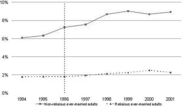
We then extend this specifi cation by adding the postreform years, plus an indica-tor for after 1996 and an interaction between religiosity and the post96 dummy. The coeffi cient on this interaction term then captures whether marital dissolution rates increased after 1996 differentially for religious versus nonreligious individuals.11 The results are presented in Section IIIA (and illustrated in Figure 2), and confi rm that, fi rst, religiosity is associated with low separation rates, and second, there was a signifi -cant increase in separations after 1996, driven by nonreligious individuals.
10. Studies in the economics of religion typically use as individual measures of religiosity either church attendance or answers to the question “How religious are you?”, see Iannaccone (1998). Our main dataset does not ask about religiosity directly, but the 2002 Irish EES survey asks about both church attendance and self- reported religiosity (on a scale from 0 to 10). Among those who report not being religious (values 0, 1, or 2), only 3.4 percent report attending church at least once a week, compared with 82.1 percent among those who report being very religious (8, 9, or 10).
11. The marital dissolution indicator takes value 1 if an individual is either separated or divorced. Figure 2
Proportion of Irish Ever- Married Adults Separated or Divorced by Religiosity, 1994–2001
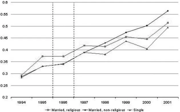
The additional identifying assumption required for religious marriages to be a valid control group is that the saving behavior of religious and nonreligious families would have followed similar trends over time, in the absence of the law change. Figure 3 provides some support for this assumption by showing that the trends in several in-dicators of saving behavior were similar for both groups in the years preceding the legalization of divorce.12 In Section IIIB we also study whether the two groups differ in a number of characteristics and discuss how we account for those differences in the regression analysis.
One could also think that single individuals would be less affected by the increase in divorce rates relative to married ones. Thus, we also use singles as an alternative com-parison group, expecting their saving behavior to be less infl uenced by the increase in marital instability.
It is of course hard to claim that either religious families or singles in Ireland were completely unaffected by the legalization of divorce.13 Moreover, Ireland during the late- 1990s experienced an economic boom which, if affecting married (nonreligious) households differentially, could provide an alternative explanation for our results. In order to address these concerns, we propose an additional control group: other Euro-pean countries undergoing similar economic conditions during the relevant period, and where divorce was already legal and no changes in the regulation of divorce took place during the 1990s.
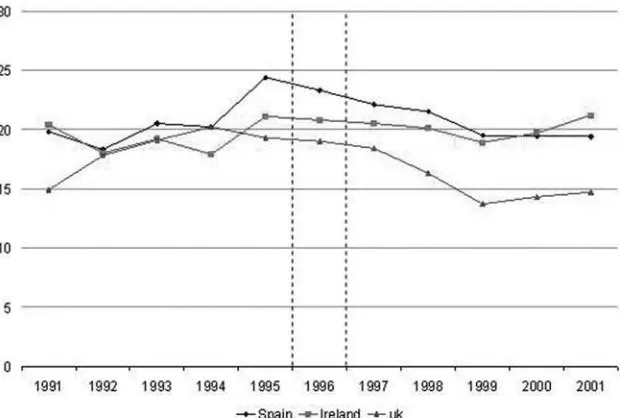
The two EU- 15 countries with more similar economic conditions to Ireland during the period appear to be the United Kingdom and Spain. In all three countries, GDP growth slowed down in 1990 and 1991, and then surged up, remaining at a higher level until 2000. That level, however, was about 8 percent for Ireland, compared with 4 percent for Spain and the United Kingdom. As for unemployment rates, they in-creased in the three countries until 1993–94, falling steadily since then, with the levels much higher in Spain than in Ireland or the United Kingdom. Figure 4 also shows that private sector savings as a percentage of GDP attained similar levels in the three countries in the early 1990s (about 18 percent in 1992), reaching a peak in 1994–95 and then declining slowly.
Although there are some differences in macroeconomic performance across the three countries, we feel the trends are similar enough to allow for the use of Spain and the United Kingdom as alternative control groups. For robustness, we also perform the analysis including additional European countries as controls.
The international comparison of saving behavior over time is carried out both using aggregate, macro data on saving rates as a percentage of GDP, and using individual- level, micro data for the different countries, which allows us to focus on the behavior of the married population as well as to include individual- level controls.
C. Econometric specifi cation and data sets
We estimate different versions of the following standard difference- in- differences specifi cation:
12. See Section IIB for the defi nition of the different saving indicators.
A. Proportion of Households Reporting Positive Weekly Savings
B. Proportion of Individuals Reporting a Savings Increase Figure 3
(2) Sijt = α+β1Tj +β2Postt+β3TjPostt+ Xijt′γ +εijt
Where S is a measure of the saving behavior (see next subsection for the specifi c vari-ables used) of an individual or household i in group j (treated or control) and year t. T is an indicator for individuals belonging in the treatment group (for instance, nonre-ligious Irish couples versus renonre-ligious ones), while Post takes value 1 for all years after divorce was legalized in Ireland. An interaction between T and Post is also included, and X stands for a set of control variables that are thought to affect savings, such as age, educational attainment and family size.14
The coeffi cient β1 measures the average difference in saving behavior between the treated and the control group, while β2 captures the overall change in saving behavior after the reform. The key parameter is β3, which indicates the change in the saving behavior of treated individuals after the reform, relative to the control group.
We estimate three sets of specifi cations, one for each control group. Our main data sets are the Living in Ireland Survey, the Irish Household Budget Survey, and the European Community Household Panel.
In the fi rst set of specifi cations, we use microlevel data for Ireland from the Liv-ing in Ireland Survey (LIS), a longitudinal household survey that covers the period 14. Some specifi cations use more than one control group, in which cases the necessary additional dummy variables and interaction terms are included.
Figure 4
Gross Private Sector Saving as percent of GDP, Ireland, Spain and United Kingdom, 1991–2001
1994–2001. The treated group in these specifi cations is composed of nonreligious marriages, and the comparison group includes religious marriages. A couple is defi ned as “religious” if both partners report going to church at least once a week in their fi rst interview, typically in 1994.15 Thus, the religiosity indicator is time- invariant for a given couple.
The main sample in these specifi cations is composed of married individuals. In or-der to avoid potential selection into marriage effects (since the legalization of divorce may well affect the incentives to marry), we exclude couples whose marriages took place in 1996 or later. In order to avoid selection due to separation or divorce, we also exclude all individuals that are observed getting separated or divorced at any point during the survey.16 Thus our married sample is in practice composed only of “stable marriages that started before 1996.” We include individuals of all ages up to 65, in order to exclude retired individuals, whose saving behavior is expected to be different. Our prereform years are 1994–96, while the postreform period spans 1997–2001. The sample size is about 2,800 married couples.
A second set of specifi cations uses single individuals as an alternative control group. When using the Living in Ireland Survey, we defi ne “singles” as individuals aged 18 to 65 who were never married in all the survey interviews.17
We also can estimate specifi cations using singles as a control group with Household Budget Survey (HBS) data, which are not longitudinal but contain much more detailed information on savings (see next subsection).18 Our prereform period includes the HBS of 1987 and 1994, while the 1999 and 2004 surveys are included in the postre-form period. When using the HBS, the sample includes all households with a head younger than the age of 64, and marital status is defi ned as the current status of the household head.
Finally, a third set of specifi cations is estimated using married couples in Ireland as the treated group and married couples in the United Kingdom and Spain as the control group. We fi rst approach the multicountry analysis by using aggregate data on saving rates as percent of GDP by country. The “treated group” in these regressions is Ireland, while the other countries serve as control group. The data on national saving rates are obtained from OECD and Eurostat publicly available fi gures.
Then, we construct an individual- level data set composed of married couples in Ireland, Spain and the United Kingdom. This multicountry, individual- level data set merges the Living in Ireland sample with the Spain and U.K. samples from the Euro-pean Community Household Panel (ECHP). The ECHP is a longitudinal survey span-ning 1994–2001 and covering all EU- 15 countries.19 In this
fi nal set of regressions, the treatment group is defi ned as married Irish individuals, the controls being married in-dividuals in Spain and the United Kingdom. Additional specifi cations use nonreligious married Irish couples as the treated group (thus religious married couples in Ireland serve as an extra comparison group). We also run specifi cations where we include
15. We explore different variations in the defi nition of “religious marriages,” see Section IIIE.
16. We also run the analysis including couples that separate in the sample (see Section IIIE). These are very few observations and whether they are included barely affects the results.
17. All LIS regressions allow for serial correlation in the error term via clustering at the individual or house-hold level (Bertrand et al. 2004).
singles in all three countries as an additional control group. The married and single samples, as well as religiosity, are defi ned as in the LIS analysis, described above.
D. Saving Variables
The literature has typically measured savings either as current income minus con-sumption, or as changes in wealth holdings over time. Both measures are deemed to be very noisy as well as subject to substantial measurement error. Our main data source, the Living in Ireland Survey, lacks good measures of either consumption or wealth. It does, however, include a range of indicators of saving behavior, both at the house-hold and the individual level. We thus use a set of binary variables that capture the propensity to save of households and individuals, but we cannot attempt to construct continuous measures of saving rates from this data source.
Fortunately, the Irish Household Budget Survey does include reasonable measures of both current income and consumption at the household level, which allows us to construct a continuous saving variable as well as to verify the quality of the informa-tion contained in the more qualitative LIS variables.
The LIS saving variables include two alternative measures of whether a household saves a positive fraction of their income. One is derived from the answer to whether the household is “able to save” (labeled “can save”), while the other is derived from a more detailed question that asks whether, considering the household’s usual income and expenses, “there is usually some money left which household members can save” (“positive weekly savings”). The second variable can be thought of as measuring the fl ow of household savings, since it follows immediately the survey questions about weekly earnings. The fi rst is phrased more vaguely and may capture either a positive stock of savings or the fl ow within a broader time span.
A third household- level saving indicator measures negative savings by indicating households that are currently repaying debt other than mortgage payments or credit card debt (“debt”). An additional debt- related variable (“debt2”) measures whether a household had to go into debt during the previous year to meet ordinary living ex-penses.
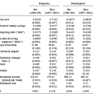
Descriptive statistics for the household- level measures of savings are shown in Table 1 (Panel A). The two binary indicators of positive household savings show signifi cant differences in levels, supporting our interpretation that they capture dif-ferent time- spans. For instance, in the prereform period, 50 percent of nonreligious households report being “able to save,” but only 32 percent report positive weekly savings.
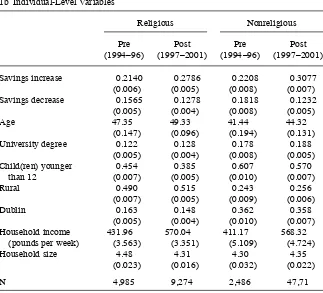
At the individual level, we use a binary indicator constructed from a question that asks whether an individual’s savings, in the bank or other fi nancial institutions, have increased over the previous 12 months (“savings increase”). This variable is closer to the standard defi nition of saving and is phrased more precisely. We also construct a binary indicator of savings decrease. Summary statistics for these variables can be found in Table 1 (Panel B). Before the reform, about 21 percent of all individuals in the sample reported an increase in their savings over the previous year, while 16 percent reported a decrease.
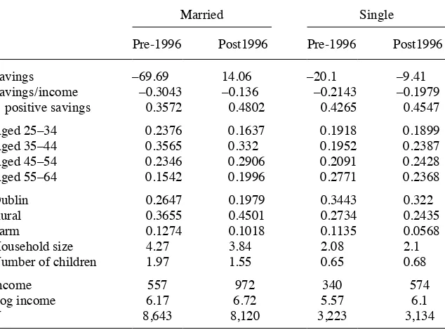
differ-ence between household income and household expenditure.20 Descriptive statistics for this variable are presented in Table 2, separately for married and single heads of household. Average savings were negative for both groups in the prereform period, and increased after 1996. Our main HBS dependent variable divides savings by total income, so that it can be interpreted as the fraction of income that a household saves 20. Both (weekly) income and consumption are reported in discrete brackets. We assign each household the middle point of the reported bracket. The income variable includes all sources of household income, and consumption includes total household expenditure. Both variables are derived from adding up the differ-ent categories of income / expenditure reported by each household. Expenditures are recorded through very detailed two- week expenditure diaries.
Table 1
Summary Statistics, Irish Married Sample (Living in Ireland Survey).
1a Household- Level Variables
Positive weekly savings 0.3406 0.4477 0.3169 0.4708
(0.008) (0.008) (0.010) (0.010)
Repaying debt (“debt”) 0.3575 0.3880 0.4433 0.4208
(0.008) (0.007) (0.011) (0.010)
In debt for living expenses (“debt2”)
0.0805 0.0491 0.1602 0.1081
(0.004) (0.003) (0.008) (0.006)
Age of husband 47.90 49.91 42.07 44.97
(weekly). On average, households in the sample save –22 percent of income, with a median of –4 percent. We also construct an indicator for positive household savings. Before the reform, 36 percent of married households had positive savings, up to 43 percent in the postreform period.
We can use this binary HBS variable to cross- check the binary saving indicators constructed from the LIS. In the 1994 HBS, 35.3 percent of married households had positive weekly savings, quite close to the 32.3 percent in the 1994–95 LIS (according to the variable “positive weekly savings”). In the 1999 HBS, the proportion is up to 43 percent, compared with 45.7 percent in the LIS variable. It thus appears that the LIS variable is reasonably accurate in measuring the proportion of households with positive savings.
As an additional check for the validity of the binary LIS variables, we calculate the correlation between each pair. The two indicators of positive household savings, “can save” and “positive weekly savings,” and the indicator for an increase in savings Table 1 (continued)
during the previous year, “savings increase,” are positively, strongly and signifi cantly correlated.21 The three indicators also have a signi
fi cant, negative correlation with the variables measuring negative savings (“debt” and “debt2”) and the indicator of a decrease in savings (“savings decrease”), which are in turn positively correlated with each other.22 We conclude that, although crude, the discrete measures of savings provided in the LIS do encode some information on households’ saving behavior.
The ECHP saving variables are essentially a subset of those in the LIS (“can save” and “debt”). Finally, the aggregate cross- country specifi cations use national saving rates as a percentage of GDP as the dependent variable. There are three measures of national savings available: gross national saving, private sector saving, and house-hold saving. Unfortunately, househouse-hold saving rates are not available for Ireland before 1996. Thus, we perform our macro- level analysis with both national saving and private sector saving rates. Figure 4 displays private sector saving rates for Ireland, Spain and the United Kingdom between 1991 and 2001.
21. For example, the correlation between “Can save”and “Positive weekly savings” is 0.54.
22. For example, the correlation between “Can save” and “Debt2” is –0.29, and between “Debt2” and “Debt,” 0.20.
Table 2
Summary Statistics, Irish Sample (Household Budget Survey)
Married Single
Pre- 1996 Post1996 Pre- 1996 Post1996
Savings –69.69 14.06 –20.1 –9.41
Savings / income –0.3043 –0.136 –0.2143 –0.1979
positive savings 0.3572 0.4802 0.4265 0.4547
Aged 25–34 0.2376 0.1637 0.1918 0.1899
Aged 35–44 0.3565 0.332 0.1952 0.2387
Aged 45–54 0.2346 0.2906 0.2091 0.2428
Aged 55–64 0.1542 0.1996 0.2771 0.2368
Dublin 0.2647 0.1979 0.3443 0.322
Rural 0.3655 0.4501 0.2734 0.2435
Farm 0.1274 0.1018 0.1135 0.0568
Household size 4.27 3.84 2.08 2.1
Number of children 1.97 1.55 0.65 0.68
Income 557 972 340 574
Log income 6.17 6.72 5.57 6.1
N 8,643 8,120 3,223 3,134
III. Results
A. The Irish divorce law and marital separation
We start by providing additional evidence that legalizing divorce increased marital separation rates in Ireland, and that the law affected nonreligious couples differen-tially. This result is fi rst illustrated descriptively in Figure 2, where we show the pro-portion of ever- married adults that were separated or divorced in Ireland between 1994 and 2001, by religiosity. The separation rate clearly increases for nonreligious adults after 1996, from about 6 percent prereform to about 9 percent in 1998–2001, while it remains around 2 percent during the whole period for nonreligious adults.
More formally, we estimate Equation 1 on the sample of ever- married adults aged 18 to 65 using LIS data. The results are presented in Table 3. The average marital separation rate (including divorces) during the 1994–2001 period was 3.8 percent, and 69 percent of the sample reported attending church at least once a week.
The fi rst column of Table 3 reports the results of estimating Equation 1 using only the prereform years (1994–96), when the average separation rate was 3.1 percent. Religiosity is the most important predictor of separation. Religious individuals are almost fi ve percentage points less likely to be separated than nonreligious ones. Living in a rural area is also associated with lower separation rates. Separation probabilities increase with age at a decreasing rate. Finally, marital dissolution is less common among the highly educated. All these factors are signifi cant, but religiosity has the highest t- value (followed by rural).
The second column adds the postreform years and includes a postreform indicator. First, note that the postreform coeffi cient is positive and signifi cant, indicating that separation rates increased signifi cantly in Ireland after 1996. Second, note also that religiosity remains strongly signifi cant. Column 3 then adds an interaction between the post96 indicator and a dummy for nonreligious individuals. Although the postreform coeffi cient remains positive and signifi cant, the interaction with nonreligious is also positive and its magnitude is larger. The separation rate increased for nonreligious individuals after 1996, both in absolute terms and relative to religious individuals.
In order to make sure that we are not just capturing a long- term trend in separation rates, Column 4 adds a linear trend, which enters positively and signifi cantly. Doing so renders the post96 coeffi cient insignifi cant, but the interaction with nonreligious remains unchanged in magnitude and signifi cance. After 1996, separation rates in-creased by 1.3 percentage points for nonreligious individuals, relative to religious ones.
Finally, in Column 5 we include some extra interactions between the postreform indicator and other factors that appear signifi cantly related to higher separation rates, such as urban residence and low educational attainment. Neither of these interaction terms attains statistical signifi cance. Moreover, their inclusion barely affects the mag-nitude or signifi cance of the religiosity interaction.
G
onz
ál
ez
a
nd Ö
zc
an
419
1994–96 All years
1 2 3 4 5
Post1996 0.0094*** 0.0056*** –0.0006 –0.0040
(0.002) (0.002) (0.003) (0.005)
Post96∗nonreligious 0.0128** 0.0128** 0.0123*
(0.006) (0.006) (0.006)
Post96∗urban 0.0026
(0.005)
Post96∗no high school 0.0034
(0.004)
Religious –0.0484*** –0.0578*** –0.0503*** –0.0501*** –0.0503***
(0.007) (0.007) (0.007) (0.007) (0.007)
Rural –0.0266*** –0.0283*** –0.0282*** –0.0282*** –0.0268***
(0.005) (0.005) (0.005) (0.005) (0.005)
Dublin –0.0103 –0.0111 –0.0110 –0.0109 –0.0109
(0.007) (0.008) (0.008) (0.008) (0.008)
Age 0.0222** 0.0133 0.0131 0.0130 0.0129
(0.009) (0.009) (0.009) (0.009) (0.009)
Age2 –0.0004** –0.0002 –0.0002 –0.0002 –0.0002
(0.0002) (0.0002) (0.0002) (0.0002) (0.0002)
T
he
J
ourna
l of H
um
an Re
sourc
es
Table 3(continued)
1994–96 All years
1 2 3 4 5
Some high school –0.0043 –0.0030 –0.0030 –0.0032 –0.0032
(0.007) (0.007) (0.007) (0.007) (0.007)
High school degree –0.0223*** –0.0225*** –0.0225*** –0.0227*** –0.0208***
(0.006) (0.007) (0.007) (0.007) (0.006)
College degree –0.0188** –0.0186** –0.0185** –0.0187** –0.0168**
(0.008) (0.008) (0.008) (0.008) (0.008)
Female 0.0321*** 0.0359*** 0.0358*** 0.0358*** 0.0358***
(0.005) (0.005) (0.005) (0.005) (0.005)
Trend 0.0015** 0.0015**
(0.001) (0.001)
Constant –0.3012** –0.1906 –0.1918 –0.1930 –0.1935
(0.124) (0.126) (0.126) (0.126) (0.126)
B. Religious families as a control group
1. Descriptives and validity of the control group
Back in Table 1 we showed some descriptive statistics for the Irish married sample, separately for religious and nonreligious households, and for the pre and postreform years.23 Nonreligious families are slightly less likely to save and more likely to be in debt than religious ones (panel a). Before the reform, 55 percent of religious families reported being able to save, compared with 50 percent of nonreligious ones. After 1996, the proportion increased for both treatment and control groups, but more so for nonreligious couples.
Panel b shows that the proportion of individuals reporting an increase in savings over the previous year was between 21 and 22 percent before the reform in both groups while the proportions with a savings decrease were 16 and 18 percent, respec-tively. After 1996, the proportion reporting that their savings were increasing rose for both groups.
Figures 3a and 3b show the year- by- year evolution of two of the main individual- level measures of saving behavior for religious and nonreligious marriages (and singles). The indicator of positive household savings (“positive weekly savings”) was slightly higher for religious families before 1996, and it displays a positive trend for both groups over the whole period. However, after 1996 it appears that the increase is steeper among nonreligious marriages. The proportion of individuals reporting in-creases in their savings evolves very similarly for all groups until 1997, but from then on nonreligious married individuals are more likely to increase their savings compared with religious marriages and singles. The next section reports the results of a more formal regression analysis.
It is important to note that religious and nonreligious households differ in a number of dimensions. Nonreligious households are younger than religious ones (by about fi ve years on average) and more educated. They are also more likely to have small children and live in Dublin, and less likely to reside in a rural area. Nonreligious families also have slightly lower income, and slightly smaller household size (age at marriage, not reported, is very similar for the two groups: 26–27). Thus, it will be important to control for these factors, since they may affect saving rates over time differentially for the two groups.
We control for age very fl exibly with a third- order polynomial. We also control for (log) household size, although the difference between the groups is small (in the preperiod, the median is 4, the 25th percentile is 3, and the 75th percentile is 5 for both groups). We also include a dummy for children younger than 12, although the difference is mostly due to the age gap between the two groups of couples. We control for education level fl exibly with four dummies, and also include dummies for Dublin and rural residence. Although the income difference is small, we control for (log) household income.24
We may worry that religious households may not only save slightly more than non-23. Religious households are defi ned as those where both partners report going to church at least once a week in the fi rst interview.
religious ones, but their saving profi le by age may differ, thus confounding our esti-mates. We calculate the proportion of households with positive savings (in 1994–96) by age, separately for control and treatment groups. The pattern is very similar, with an increasing propensity to save in the late 20s, a decline in the early 30s, a second peak around the mid- 50s and a decline from then on.25 In any case, we also estimate specifi cations that include interactions between the age polynomial (as well as the rest of the controls) and religiosity. We believe this allows us to correct for the potential effect of differences in the stage in the life cycle between the two groups.
2. Regression Results
The main regression results for the individual and household sample are reported in Tables 4 and 5. Table 4 focuses on the binary dependent variable “can save.” Results are reported for several different specifi cations. Columns 1–4 include only the married sample. The fi rst specifi cation includes no control variables, thus the results can be interpreted as pure differences in means. Married households were signifi cantly more likely to save after 1996, while religious families saved more than nonreligious ones. After 1996, nonreligious families increased their propensity to save by almost three percentage points, relative to religious ones.
Column 2 adds a full set of control variables, including age, age squared, age cubed, educational attainment dummies, log household size, log income, a dummy for chil-dren younger than 12, and rural and Dublin indicators (coeffi cients not reported).26 We also include year dummies, in order to control for the effect of overall economic conditions.27 The coef
fi cient of interest remains signifi cant and increases in size. More educated and higher- income households are signifi cantly more likely to save, while larger families are less likely to. Dublin residents save more, as do families with young children. The year dummies are not signifi cant, and neither is age once all the other controls are included. The effect of interest is now estimated at almost four percentage points.
Column 3 reports the results from a specifi cation that interacts the year dummies with a religiosity indicator. This turns the coeffi cient of interest even larger, at almost seven points. Finally, Column 4 includes all the controls as well as household fi xed- effects, our preferred specifi cation. Even in this saturated specifi cation, the estimated effect is a signifi cant four percentage points (for an average saving propensity of 63 percent). As a benchmark to assess the magnitude of the effect, the difference in the proportion of couples “able to save” between those with a high school versus a college graduate husband is about seven percentage points.
Table 5 reports the coeffi cients on the interaction term between “post” and “non-religious” for four additional dependent variables and several different specifi cations. Each row now reports the results for a different outcome variable. Columns 1 and 2 show the results when using religious couples as the control group (without and with household fi xed effects, respectively). The results go in the same direction as 25. These results are available upon request from the authors.
26. Some of the control variables, such as income, could be determined endogenously, which calls for some caution when interpreting these results.
G
Treated*post 0.0288 0.0374** 0.0665** 0.0399** 0.0178* 0.0323**
(0.0184) (0.0173) (0.0293) (0.0189) (0.0107) (0.0153) Specifi cation Linear probability
model (LPM)
LPM LPM LPM with household
fi xed- effects
LPM LPM with household fi xed- effects
N 12,698 12,675 12,675 12,675 29,690 29,690
those in Table 4. The second indicator of a household’s propensity to save (“posi-tive weekly savings”) increased by 4–6 percentage points more for treated rela(“posi-tive to control families after divorce was legalized. We also fi nd that nonreligious families were signifi cantly less likely to be in debt after the reform, relative to religious ones, by 6–7 percentage points when we use the indicator for repaying debt and by about three when we look at whether the household had to incur in debt to pay for its usual expenses. Finally, we estimate that nonreligious families were about three percentage points more likely to report a savings increase during the previous year after 1996, relative to religious marriages.
One may also be interested in the timing of the estimated effects. We run additional specifi cations where we interact nonreligious marriages with each single year after Table 5
The Impact of Legalizing Divorce on Household Saving, Irish Household Sample, Five Dependent Variables
Note: Living in Ireland Survey data. [Positive weekly savings: Household can usually save weekly; Debt: Household is repaying debt; Debt2: Household indebted last year to pay ordinary living expenses.] The
1996, instead of with a single postreform indicator.28 The coeffi cient estimates suggest that the effects increase over time for the three main measures of saving behavior. In 1997, the effects are small and insignifi cant. The estimated effects become signifi cant in 1998–99, and their magnitude peaks in 2000–2001. Note that this pattern follows closely the timing of increase in the divorce rate (see Figure 2).
In sum, we fi nd that married individuals in Ireland were more likely to save after 1996, and this increase was signifi cantly higher among nonreligious couples. Non-religious households were also less likely to incur debt relative to Non-religious married households. The results suggest that nonreligious married people in Ireland increased their savings (relative to more religious people) after 1996, the time when divorce was legalized.
C. Singles as a control group
Next, we turn to singles as an alternative control group (while all married couples are included in the treated group). The advantage of this second comparison group is that we can exploit Household Budget Survey data, which allows us to construct a continu-ous measure of savings from income and expenditure information.
We fi rst report specifi cations using LIS data for the same set of dependent vari-ables used in the previous section. Singles are signifi cantly younger than the married sample, with average age of 27 compared with 47 for married individuals. Singles are also much more likely to hold a high school degree, live in smaller households, are less likely to have small children and have higher income. The proportion living in rural areas and Dublin is similar for married and singles.29
The regression results are reported in the last two columns of Tables 4 and 5. Table 4 (Column 6) shows that married couples increased their propensity to save by about three percentage points after 1996, relative to singles, and this difference is signifi cant. Table 5 (Columns 3 and 4) suggests that these effects are also present in the remain-ing dependent variables. Married couples are signifi cantly less likely to incur in debt after 1996 relative to singles, and they are signifi cantly more likely to increase their savings.
Although the Irish Household Budget Survey has no information on religiosity, it does contain information on marital status. Thus, we can estimate our specifi cation using singles as the control group for the continuous variables of savings constructed from HBS data. The descriptive statistics for the HBS sample were reported in Table 2. As noted earlier, average savings are negative for both samples before 1996, and they increase over time. Note that the prereform period now includes data from 1987 and 1994, while the post1996 data come from the 1999 and 2004 surveys. All specifi ca-tions include year dummies.
The main regression results are presented in Table 6, using the saving rate (savings divided by income) as the dependent variable.30 The coeffi cient of interest is, as be-fore, the interaction between the married indicator and the post1996 dummy. Column 1 in Table 6 shows the results when including the full set of controls, except household
28. These results are available upon request from the authors.
T
The Impact of Legalizing Divorce on Household Saving Rate, HBS Irish Sample
1 2 3 4 5 6 7 8 9
Married∗Post96 0.1594*** 0.0847** 0.2482*** 0.0733 0.2554*** 0.0682*** 0.0534*** 0.0913*** 0.0439** (0.0422) (0.0391) (0.0608) (0.0564) (0.0615) (0.0135) (0.0122) (0.0161) (0.0174) Married –0.1562*** –0.3302*** –0.1992*** –0.3448*** –0.1782 –0.0677*** –0.1244*** –0,0472*** –0,0914***
(0.0364) (0.0339) (0.0480) (0.0445) (0.2031) (0.0116) (0.0106) (0.0128) (0.0138) 1994 0.0462* –0.1415*** –0.0121 –0.1621*** 0.0021 –0.0128 –0.0697*** 0.0145 –0,0238* (0.0262) (0.0245) (0.0504) (0.0467) (0.0506) (0.0084) (0.0077) (0.0134) (0.0144) 1999 0.0186 –0.4674*** 0.0198 –0.4978*** 0.0223 –0.0060 –0.1566*** 0.0338** –0,1076***
(0.0410) (0.0388) (0.0519) (0.0489) (0.0523) (0.0131) (0.0121) (0.0138) (0.0151) 2004 0.0538 –0.6511*** –0.0107 –0.6439*** –0.0054 0.0612*** –0.1544*** 0.0403*** –0,1442***
(0.0410) (0.0396) (0.0518) (0.0491) (0.0524) (0.0131) (0.0124) (0.0138) (0.0152)
Married∗1994 0.0801 0.0281 0.0730 –0,0428*** –0,0567***
(0.0591) (0.0547) (0.0592) (0.0157) (0.0169)
Married∗1999 –0.0913 0.0523 –0.0877 –0,0802*** –0,0502***
(0.0598) (0.0555) (0.0602) (0.0159) (0.0171)
income (since it is potentially endogenous). We fi nd that married households increased their savings by 16 percentage points after 1996, relative to single households. When we control for log income (in Column 2), the estimated effect falls to a still signifi cant 8.5 points. Note that income enters the regression with a positive and signifi cant coef-fi cient, capturing the fact that richer households tend to save a higher fraction of their income. The fact that the coeffi cient of interest falls when income is included suggests that the increase in savings among married couples after the reform is in part due to higher income.
We run additional specifi cations where we interact the married indicator with the year dummies (in Columns 3 and 4), with similar results (but lower precision).31 In Column 5, we also interact all the controls with the married indicator, to allow for different coeffi cients on age, education, etc, for the married and single sample. The coeffi cient of interest remains large and signifi cant.
Finally, one may worry that outliers could be driving the results, since the distribu-tion of saving rates is severely skewed to the left. Thus, we estimate median regres-sions (parallel to Columns 1–4), shown in Columns 6–9, which should minimize the impact of outliers. These specifi cations suggest that the saving rate of married couples increased signifi cantly after 1996, by 5–9 percentage points. As a benchmark to assess the magnitude of our estimated effects, the average saving rate in the sample increased by almost 17 percentage points between 1987 and 2004.
We also estimate specifi cations using raw savings as the dependent variable (with-out dividing by income) and using the binary indicator of positive savings (for com-parability with the LIS results). We fi nd that married couples increased their savings by 50–70 euros a week after 1996 (signifi cantly), relative to single households. The fraction of married households with positive savings increased (signifi cantly) by 7–9 percentage points, relative to singles.32
Thus, we conclude that married couples in Ireland increased their propensity to save signifi cantly after 1996, relative to single individuals. We now turn to our third ap-proach, where we use married couples in other countries as additional control groups.
D. Other countries as control groups
1. Aggregate data analysis
The evolution of the private saving rate as a percentage of GDP in Ireland, Spain and the United Kingdom between 1991 and 2001 can be found in Figure 4. This period covers fi ve years before and fi ve years after the legalization of divorce in Ireland. In the mid- 1990s, all three countries had private saving rates around 20 percent of GDP. We estimate simple difference- in- difference specifi cations following Equation 2, where the dependent variable is the log of the private saving rate, and report the results in Table 7 (Columns 1–3). The fi rst column includes only the United Kingdom as a control country, while the second adds Spain and the third also includes France and Germany.
On average, private savings declined after 1996 for the three sets of countries.
How-31. The interaction terms between married and the year dummies are not jointly signifi cant in specifi cations 3 or 4.
T
he
J
ourna
l of H
um
an Re
sourc
es
Table 7
Aggregate Saving Rate Results
Log Private Saving Rate Log Aggregate National Saving Rate
1 2 3 4 5 6 7
Post1996 –0.1586* –0.1051* –0.0628*** –0.0711 –0.0383 –0.0088 –0.0233
(0.0844) (0.0616) (0.0417) (0.0811) (0.0581) (0.0458) (0.0431)
Ireland∗Post1996 0.1443* 0.0997* 0.0833* 0.2443*** 0.2322*** 0.2648*** 0.2983***
(0.0718) (0.0583) (0.0477) (0.0581) (0.0457) (0.0432) (0.0466)
N 26 39 65 28 42 70 98
Years 1989–2001 1989–2002
Control countries United Kingdom
United Kingdom, Spain
United Kingdom, Spain, Germany, France
United Kingdom
United Kingdom, Spain
United Kingdom, Spain, Germany, France
United Kingdom, Spain, Germany, France, Italy, Portugal
ever, relative to the control countries, private savings increased signifi cantly in Ireland after 1996. The size of this (relative) increase was about 14 log- points relative to the United Kingdom, down to 10 when including Spain as an additional control, and eight when adding Germany and France.33
The results of specifi cations that use the log of the aggregate national saving rate as a dependent variable are reported in Columns 4–7. The results show that the Irish saving rate increased after 1996 by 24 log- points relative to the United Kingdom (Column 4). The size of the estimated effect remains almost unchanged when we include additional control countries: Spain (Column 5), France and Germany (Column 6), and fi nally also Italy and Portugal (Column 7). The estimated effects are strongly signifi cant.34
Thus, we fi nd that the saving rate in Ireland increased signifi cantly after 1996, and this increase was signifi cantly higher than that in other European countries (where in fact saving rates were stable or declining). The next subsection provides some evidence that this relative increase in saving rates may have been related to the 1996 legalization of divorce.
2. Individual- level, multicountry analysis
Table 8 shows some summary statistics for the three- country sample (using LIS data for Ireland and ECHP for Spain and the United Kingdom), separately for Ireland,
33. We also run specifi cations that include a linear time trend, but the trend is never signifi cant at the 10 percent level and its inclusion barely changes the magnitude of the estimated effects.
34. Including linear trends in all specifi cations does not signifi cantly alter the results, and the trend is typi-cally not signifi cant.
Table 8
Summary Statistics, Three- Country Married Sample
Ireland Spain United Kingdom
Pre Post Pre Post Pre Post
Save 0.3326 0.4558 0.3469 0.4621 0.6820 0.7214
Debt 0.3864 0.3995 0.2601 0.2599 0.3999 0.3759
Age 45.94 48.18 46.02 47.55 44.93 47.29
University degree 0.155 0.164 0.177 0.191 0.388 0.506
Household income
(euros) 25,381 33,557 16,637 20,241 25,149 38,498
Household size 4.43 4.38 3.93 3.95 3.32 3.38
N 5,962 6,736 11,387 12,380 4,739 6,688
Spain and the United Kingdom and for the pre and postreform periods. Before the reform, saving rates were much higher in the United Kingdom than in Ireland or Spain (68 percent compared with 33–35 percent). Before 1997, saving rates were increasing both in Ireland and in Spain, although the increase was steeper in Spain. The propor-tion of households in debt before the reform was lowest in Spain.
The age profi le is similar in the three countries while income levels (in euros) were similar in the United Kingdom and Ireland but signifi cantly lower in Spain. Household size was highest in Ireland. After 1996, the propensity to save increased in all three countries while the proportion of households in debt remained essentially fl at.
The main regression results for the three- country sample are reported in Table 9. The control variables show similar patterns as in the Irish sample. Higher education is associated with a higher propensity to save and a lower likelihood of being in debt, while the age profi le has low signifi cance levels.
After 1996, the propensity to save of married couples increased in Ireland by 3–4 percentage points, relative to the United Kingdom and Spain, and this effect was sig-nifi cant (Table 8, Columns 1 and 2). In fact, this effect is mostly driven by the com-parison to the United Kingdom. When including only the United Kingdom as a control country, the estimated effect is a signifi cant nine percentage points, while it is only a less signifi cant two points relative to Spain (not shown).
Columns 3 and 4 show the results when using nonreligious Irish couples as the treated group. Since the ECHP does not include the church attendance variable, we cannot separate couples by religiosity in the United Kingdom and Spain. These speci-fi cations also include an indicator for Ireland interacted with nonreligious (not re-ported). The results show that married couples were more likely to save in Ireland after 1996 relative to the other countries but this increase was more pronounced among nonreligious households. The estimated effect is between four and fi ve percentage points.
Finally, the last two columns show the results when including singles as an addi-tional control group.35 These regressions now include a dummy for married interacted with each country, plus an indicator for married interacted with post1996 (common for all countries), the interaction between Ireland and nonreligious marriages, and the quadruple interaction of Ireland, married, nonreligious and post. The results show that married individuals save more than singles in all three countries (not reported), while savings increased overall after 1996, and signifi cantly more for married individuals relative to singles (not reported). We also fi nd that the increase in the propensity to save was signifi cantly more pronounced in Ireland (by about seven percentage points). Moreover, nonreligious married individuals in Ireland increased their propensity to save more than religious couples and singles in Ireland, relative to the other countries, by about fi ve percentage points.
We also estimate specifi cations for the second dependent variable (a binary indica-tor for debt). We fi nd that nonreligious marriages in Ireland were less likely to be in debt after 1996, relative to the control group of singles and religious couples in Ireland as well as married and single households in the United Kingdom and Spain.36
G
Post1996 0.0482*** 0.0693*** 0.0483*** 0.0693*** 0.0422*** –0.0018
(0.0056) (0.0053) (0.0056) (0.0053) (0.0048) (0.0052)
Ireland∗Post 0.0271*** 0.0443*** 0.0101 0.0306** 0.0767*** 0.0637***
(0.0103) (0.0110) (0.0122) (0.0133) (0.0088) (0.0092)
Ireland∗Post∗Nonrel. 0.0507*** 0.0398**
(0.0183) (0.0199)
Ireland∗Post∗Nonrel.∗Married 0.048*** 0.0476***
(0.0178) (0.0183) Treated group Married couples in Ireland Nonreligious marriages in
Ireland
Nonreligious marriages in Ireland
Control group Married couples in United Kingdom and Spain
Control variables All None All None All None
Specifi cation LPM LPM w.
N 47892 47892 47892 47892 106636 106636
Note: The married sample includes all couples married before 1996 and never separated or divorced in Spain, the United Kingdom and Ireland. The singles sample includes all never married individuals who do not change marital status in Spain, the United Kingdom and Ireland. Standard errors clustered by household are in parentheses. * = 90 percent confi dence level; ** = 95 percent, and *** = 99 percent. All specifi cations include country dummies. Specs. 3 to 6 also include a dummy for Ireland∗Nonreligious. Specifi cations 5 and 6 also include dummies for Married∗country, Married∗post, and Ireland∗post∗married. “All” controls include age, educational attainment, log household
E. Additional specifi cations and robustness checks
We have estimated a number of alternative specifi cations as robustness checks.37 We explored some variations in the sample selection and the control variables included. For instance, we selected the sample based on the age of the husband or on the age of the wife, and included as a control the age of the husband, the age of the wife, or both at once. These variations made little difference in the results.
Given the economic boom experienced by Ireland during the 1990s, we tried ad-ditional specifi cations in order to discard that economic growth could be the main driver of our results. We estimated all regressions including controls for aggregate economic conditions, such as the aggregate unemployment rate. This barely affected the coeffi cient of interest, suggesting that differences in timing allow us to separate the effect of the divorce law from that of the contemporaneous economic boom. We also estimated regressions controlling for income at the household level (already shown in the main tables), as well as an additional set that also controlled for wives’ employ-ment, since growth could have affected female labor supply differentially for married (nonreligious) women. This again made little difference to the results.
Of course, household income and labor supply are both endogenous and could well have reacted to the legalization of divorce. Moreover, it is useful in itself to investigate whether the increase in savings by married couples that we fi nd took place via in-creases in income or reductions in consumption. Thus, we estimate regressions parallel to those shown in Tables 4–6, but using household income and expenditure as the de-pendent variables, in turn. The results suggest that income reacted little to the reform, while affected couples appeared to reduce their expenditures after the policy change.
Also relevant are the specifi cations for the LIS sample that used alternative defi nitions of religiosity. Our main defi nition of “untreated” household includes couples where both husband and wife report going to church at least once a week in the fi rst interview (66 percent of the married sample). A more strict defi nition would include couples where both report going to church more than once a week, but that would account for only about 5 percent of the sample. A less strict defi nition would include couples where at least one of them goes to church once a week, but this would include almost 99 percent of married households. Finally, we could classify as religious couples those where both report going to church at least once a month (76 percent of the sample). Using this less strict defi nition barely alters the magnitude of the estimated effects, which become slightly stronger for some of the dependent variables, as expected.38
The main specifi cation using the LIS sample excludes couples who end up divorc-ing or separatdivorc-ing by 2001. When we estimate specifi cations that include the separating couples, the effect typically gets stronger; indicating that those households adjust their saving behavior (while still married) more than the couples who do not break up, as expected. However, we observe few separations in the data, which may explain why the size of the coeffi cient only changes slightly.
The baseline LIS results include all years between 1994 and 2001, but we also try 37. Regression results for all the specifi cations in this section are available upon request.
dropping years 1996 and 1997, the “reform years.” This weakens the estimated effects slightly, but they remain mostly signifi cant.
Finally, when using families in other countries as comparison groups, we explored using only Spain and only the United Kingdom as control countries.39 The estimated effect was smaller and less signifi cant when using only Spain as a control country.
IV. Conclusions
We have shown that the propensity to save of married couples in-creased signifi cantly in Ireland after 1996, relative to singles (and to married couples in other European countries). This increase was signifi cantly higher among nonreli-gious married couples, compared with relinonreli-gious ones. One possible reason for this increase in the propensity to save of Irish married individuals is the legalization of divorce that took place in 1996, which increased the risk of marital breakup, espe-cially for nonreligious families. These results are consistent with married individuals increasing their savings in anticipation of a potential divorce.
We estimate that an increase in the risk of marital separation of about 40 percent (among nonreligious marriages) led to a signifi cant rise in the proportion of married households reporting positive savings (of 7–8 percent or 10–13 percent, depending on the saving indicator used). Nonreligious married couples also were about 11 percent more likely to report that their overall savings had increased over the previous year. Rel-ative to singles, the proportion of married couples reporting positive savings increased by 4–5 percent, and their savings as a proportion of income increased by 5–8 percent.
Some caveats of our analysis are worth mentioning. First, in an important part of our individual- level analysis we are only able to use binary indicators of saving activity, which makes it hard to draw quantitative conclusions about changes in the individual saving rate. Second, we lack a true control group within Ireland, thus our analysis uses alternative “comparison groups,” but the results may understate the true effect if the comparison group is also partially affected by the legal change. And third, we only have access to few prereform years, and are thus unable to control for long- term prereform trends, which would strengthen our identifi cation strategy.
Nevertheless, our results that married couples affected by the legalization of divorce increased their savings after the reform are consistent when using three different control groups (religious couples, singles, and married couples in other countries) and across three independent data sets (LIS, HBS and ECHP) and eight different measures of sav-ing behavior. The main results are also robust to a number of specifi cation checks, and do not seem to be driven by the overall improvement in economic conditions in Ireland.
The fi ndings suggest that divorce legislation may affect not only marital breakup rates and the income of individuals directly affected by a divorce, but also the eco-nomic behavior of individuals who stay married, who may adjust to the change in the risk of future marital separation. Previous studies have suggested that one channel of adjustment is likely to be labor supply,40 and we provide evidence that saving behavior may also adjust signifi cantly.
39. We also explored using all other EU15 countries as controls.