The Effect of a Health and Family Planning
Program on Out- Migration Patterns
in Bangladesh
Tania Barham
Randall Kuhn
Barham and Kuhnabstract
There is concern that benefi t programs may alter out- migration patterns. We exploit the quasi- random placement of a health and family planning program in Bangladesh to examine changes in out- migration patterns. Using individual- level migration data from 1979–91, we fi nd that the fl ow of out- migration was approximately 15 percent lower for women and men in the treatment versus comparison area. We fi nd comparable changes in out- migrant stock, showing that effects persisted even after allowing for return migration. Our fi ndings suggest that benefi t programs can lead to longer run changes in population, with consequences for program evaluation design and economic development.
I. Introduction
Migration fl ows are generally thought to be essential to the effi ciency of national economies, and there is concern that government programs or development aid could alter the fl ow by changing the relative income between areas. In particular, there has been a long debate in the United States on the extent of welfare- induced
Tania Barham is an associate professor of economics and Institute of Behavioral Science faculty at the University of Colorado Boulder. Randall Kuhn is an associate professor and Director of the Global Health Affairs Program in the Josef Korbel School of International Studies at the University of Denver. The authors are grateful to Brian Cadena, Richard Jessor, and Terra McKinnish for their helpful comments, and to Gisella Kagy for her research assistance. The authors thank the ICDDR,B Health and Demographic Surveillance Unit for providing the Health and Demographic Surveillance System data. In particular, the authors thank Sajal Saha, Abdur Razzaque, Nizam Khan, and Khairul Islam for their help in preparing and understanding the data and Dr. Mohammad Yunus and Mr. J. Chakraborty for information on the rollout of the Matlab Maternal and Child Health and Family Planning program. The data are available from ICDDR,B by request. The authors are willing to advise other scholars on acquisition.
[Submitted June 2013; accepted October 2013]
ISSN 0022-166X E- ISSN 1548-8004 © 2014 by the Board of Regents of the University of Wisconsin System
migration and whether or not high- benefi t areas are “welfare magnets” (Cebula 1979; Moffi tt 1992). In developing countries, there is a need to understand what prevents rural populations from migrating to fi nd better jobs (Ardington, Case, and Hosegood 2009), and if targeted aid to rural areas slows migration to more prosperous areas (Chen et al. 1998; NRC 2003).
Determining how migration responds to benefi t programs is clearly important but estimating the causal effect is challenging. Many government benefi ts are set federally and therefore lack within- country variation. Where within- country variation exists, it is usually not exogenous, making it challenging to identify good counterfactual groups and leaving concerns that unobservables may be biasing results or that ben-efi t levels may be endogenously set. In addition, migration effects can be diffi cult to estimate since migration rates are often very low, sample sizes too small, or the data too aggregated to capture changes in migration (Moffi tt 1992; Gelbach 2004). As a result, rigorous research examining the migration response to programs that provide important cash or noncash benefi ts is sparse.
To address the above- noted challenges, we exploit the quasi- random placement of an important nongovernmental health program—The Matlab Maternal and Child Health and Family Planning (MCH- FP) program—in the rural Bangladesh district of Matlab. We estimate the causal effect of this program on the fl ow and stock of out- migrants from Matlab. This program arguably included some of the most important health interventions in the latter part of the twentieth century: family planning and childhood vaccination. The program was especially valuable to the local population because it provided access to health services, such as vaccines, that were diffi cult to obtain through government clinics. Previous research has shown that the MCH- FP program had benefi cial effects on several dimensions of human capital accumulation including reductions in child mortality and fertility (Phillips et al. 1982, 1984; Koenig et al. 1990, 1991) and long- term improvements in cognitive functioning, height, and education (Barham 2012; Joshi and Schulz 2013). The program was phased- in start-ing with family plannstart-ing in late 1977, followed by child health interventions in 1982, with many of the health interventions becoming available in the comparison area after 1988. This phasing- in provides three time periods in which to examine program ef-fects: 1979–81, 1982–88, and 1989–91.
This study benefi ts from unusually rich data from a long- term Health and Demo-graphic Surveillance System in Matlab that regularly collects a variety of data in-cluding prospective observation of migration events. Using individual- level data from 1979–91, we estimate the short- term program effects with age and year fi xed effects on the fl ow and stock of out- migration from the area. Our analysis focuses on women aged 25–44 and men aged 30–49 because they are more likely to be married, to benefi t from program interventions, and to focus on the potential short- term effects of the program on adult labor migration rather than on marriage migration. As a falsifi cation check, we also examine program effects for 19–22- year- olds. We focus on the fol-lowup period through 1991 in order to isolate the short- term effects of the program on the value of living in an area with improved health and family planning services from longer- run changes resulting from the effects of the program itself on, for example, human capital, family size, and population size.
MCH- FP program on the share of people who migrated out of the study area that year. To take account of the many out- migrants that return to the study area, we also follow a cohort of people that was in the sample age range in the fi rst year of the program and use panel data to examine the effect of the program on the stock of out- migrants (for example, the share of individuals, present at the start of the program, living outside the area in a given year).
The MCH- FP program was quasi- randomly assigned and a comparison group built into the design of the program. This design enables the use of a single difference estimator to evaluate the change in the fl ow and stock of out- migrants between the treatment and comparisons areas for the three study time periods. Unfortunately, we lack adequate migration data to understand if there were any differences in migration rates between the two areas prior to program inception. Therefore, to be conservative, we use the fi rst study period (1979–81), when only some of the program services were available, as a baseline to estimate double- difference program effects for the latter two study time periods. The available preprogram data are used to show that the treatment and comparison groups are similar with respect to most other observable characteristics at baseline.
We fi nd the program did not lead to statistically signifi cant differences in the fl ow of out- migrants between the treatment and comparison area in the 1979–81 period. How-ever, during the middle time period, the fl ow of out- migrants was 15 percent lower for women and 17 percent lower for men in the treatment compared to the comparison area for total migration (combined domestic and international). The program effect was slightly larger for domestic migration, 19–21 percent, and there was no statisti-cally signifi cant effect on international migration. During the 1989–91 period, when health services were expanded in the comparison area, program effects were lower and generally not statistically signifi cant. After allowing for return migration, the stock of out- migrants was still lower in the treatment than the comparison area for both women and men during the 1989–91 period.
This paper adds to an important but sparse literature estimating causal effects of various types of benefi t programs on migration patterns. For example, recent research on welfare migration in the United States has exploited differences in the generosity of cash welfare benefi ts across states. The research shows that the effect of welfare migration on people most likely to benefi t—single mothers without a high school degree—is fairly modest (Gelbach 2004; McKinnish 2005, 2007).1 In Mexico and
Nicaragua, research that examined the effect of randomized conditional cash transfer programs on behavioral responses, including migration of older teens and prime- age adults, yielded mixed results. In Mexico, the program led to a decrease or no im-pact on domestic migration but a small increase in international migration (Angelucci 2012; Stecklov et al. 2005),2 while in Nicaragua there was an increase in migration of
1. For a review of the welfare migration literature prior to the1990s, see Cebula (1979) and Moffi tt (1992); for reviews of the more recent literature, see Gelbach (2004) and McKinnish (2007).
males across a wide age range (Winters, Stecklov, and Todd 2006).3 In South Africa,
Ardington, Case, and Hosegood (2009) used longitudinal data to examine the effect of a household member gaining or losing an old- age pension on labor migration of prime- age adults living in the same household. They found that an increase in pension income leads to a small increase in labor migration, but they did not examine the effect on domestic and international migration separately.
This paper advances research on program- induced migration in several respects. First, we exploit a quasi- random experiment that benefi ts from having treatment and comparison groups, relatively large sample sizes, and prospective individual- level migration data. This design enables us to address many of the methodological de-fi ciencies in the literature. Second, most previous research has focused on programs that provide cash benefi ts rather than direct service provision. Direct service programs are widespread in both developed and developing countries, and constitute a greater share of expenditure than do cash welfare programs in many countries, and therefore are important to examine. Third, the duration of the migration data series allows us to measure the persistence of the treatment- comparison migration differential across more than a decade. Such a long duration allows us to account for the effects of re-turn migration on the out- migrant stock over time. Importantly, the examination of the stock of out- migrants provides insight into the extent of attrition bias that may be present in long- term evaluations of similar programs. While the results are not valid beyond the study site, the program benefi ted people across the socioeconomic spectrum so might provide insight into possible migration responses to similar health interventions in countries with levels of development comparable to those in Matlab and potentially among the poor in developed countries.
The remainder of this paper proceeds as follows. Section II provides a brief descrip-tion of the MCH- FP program and the mechanisms through which the program may affect migration; Section III describes the data; Section IV explains the identifi cation and estimation strategy; the fi ndings and robustness analysis are discussed in Section V; and Section VI concludes.
II. Background
A. Overview of the Matlab MCH- FP Program
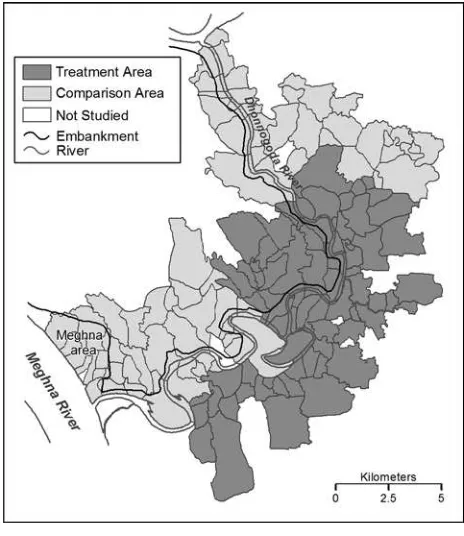
The International Centre for Diarrheal Disease Research, Bangladesh (ICDDR,B) began the MCH- FP program in Matlab in October 1977 as a demonstration project to help the government design its national family planning program. Approximately 200,000 people in 149 villages were fairly evenly split between treatment and compar-ison areas (Figure 1). The program included integrated family planning and maternal and child health services. Service delivery was intensive as interventions were ad-ministered in the house of the benefi ciary during monthly visits made by local female
health workers hired and trained by the program (Bhatia et al. 1980). These services were offered free of charge.
Health and family planning services were also available in government clinics in the area, but there was limited or no home delivery. In addition, many of the services provided by the MCH- FP program, such as childhood vaccinations, became readily available from the government only after 1988, thus providing an experimental period between 1977–88 to evaluate the program. Evaluation of the program is also aided by the phasing in of program services over two main periods: 1977–81 and 1982–88.
Program services in 1977–81 focused on family planning and maternal health through the provision of modern contraception,4 tetanus toxoid vaccinations for
nant women, and iron and folic acid tablets for women in the last trimester of preg-nancy (Bhatia et al. 1980). Female health workers provided in- home counseling on contraceptives, nutrition, hygiene, and breastfeeding. They also motivated women to continue using contraceptives, and instructed them on how to prepare oral rehydration
4. Contraceptive methods provided in the home included: condoms, oral pills, vaginal foam tablets, and injectables. Methods provided at program health clinics included: intrauterine device insertion, tubectomy, and menstrual regulation.
Figure 1
Map of Matlab Study Area
solution. These services were supported by a followup and referral system to ensure management of side effects and continued use of contraceptives (Phillips et al. 1984; Fauveau et al. 1994).
Between 1982–88, additional interventions were provided in the treatment area, especially for children younger than age fi ve. The measles vaccine was provided in half the treatment area beginning in 1982. Starting in 1985, services were rolled out to children younger than the age of fi ve in the entire treatment area, including four essential vaccines5, Vitamin A supplementation, and curative care such as nutrition
rehabilitation and acute care for respiratory infections. In addition, the tetanus toxoid immunization was expanded to all women of reproductive age and safe delivery kits were provided to pregnant women.
The program is still running today but differences between the treatment area and the rest of the country, including the comparison area, diminished after 1988 as the les-sons from the success of the Matlab MCH- FP program were incorporated into the na-tional plan (Phillips et al. 2003; Cleland et al. 1994). In particular, Bangladesh greatly increased the number of family welfare assistants to deliver in- home contraceptive and immunization services throughout the country. Expanding the number of family welfare assistants reduced the client- worker ratio from 1 per 8000 in 1987–88 to 1 per 5,000 in 1989–90 (Cleland et al. 1994). The ratio was still lower in the treatment area at 1 per 1,300 in 1990.6 Improvements in supply chains, products, and management
were also rolled out in 1988 and 1989 (Cleland et al. 1994).
B. Program Implementation
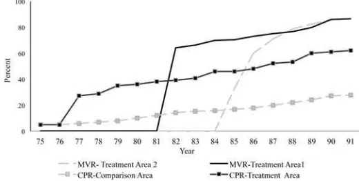
Program implementation followed the planned timeline, and the subsequent uptake of interventions was rapid. For example, Figure 2 shows that the contraceptive preva-lence rate (CPR) for married women aged 15–49 in both the treatment and comparison areas was similarly low prior to the introduction of the program (less than 6 percent). There was a large increase in the CPR to 30 percent in the treatment area during the fi rst year of the project (1978). After that, there was a steady increase in the CPR, reaching almost 50 percent by 1988. Due to availability of contraceptives from gov-ernment services in the comparison area, the CPR increased in the comparison area over time, but not as quickly, and rates remained below 20 percent in 1988. There was still a 20 percent difference in the CPR rate between the two areas in 1991.
Figure 2 shows the measles vaccination rate also rapidly increased from approxi-mately 0 to 60 percent in 1982 after it was introduced in the fi rst half of the treatment area (Treatment Area 1), and in 1985 when it was introduced in the other half of the treatment area (Treatment Area 2). Vaccination rates in the comparison area are not documented for this time period but are believed to be near zero. Government services did not regularly provide the vaccines for children until around 1989, so the population in the comparison area is viewed as being largely unvaccinated prior to 1989 (Koenig,
5. Measles, polio, tuberculosis, and diphtheria, pertussis, tetanus (DPT).
Fauveau, and Wojtyniak 1991). The measles vaccination rate for children younger than the age of fi ve was less than 2 percent nationally in 1986 (Kahn and Yoder 1998), and was below 40 percent in the comparison area in 1990 (Fauveau 1994). As the national vaccination program scaled up, the difference in vaccination rates between the treat-ment and comparison area narrowed substantially but not completely. For example, by 1988 in the treatment area, vaccination rates for children aged 12–23 months were 88 percent for measles, 93 percent for tuberculosis, 83 percent for all three doses of DPT and polio, and 77 percent for all three major immunizations (HDSS 2007). In the comparison area, according to data from the 1996 Matlab Health and Socioeconomic Survey, the vaccination rates for children born in 1991 reached 78 percent for measles and 60 percent for the third dose of DPT.
C. Potential Effect of the MCH- FP Program on Migration
Whether a program alters short- term migration patterns depends on a number of fac-tors. These include how much the benefi ciaries value the program, specifi cs of the program including whether or not it requires the recipient to be physically present to receive benefi ts, and the mechanisms that drive migration. Based on the description of the program interventions in Section IIA, the individuals or families most likely to value or benefi t from the MCH- FP program are: those who are married (since premari-tal sexual activity is rare among Bangladeshi women), those in need of ongoing family planning services or maternal care, and those with children younger than the age of fi ve.7 With the exception of a few contraceptive methods, program services were
al-7. It is possible that the program affected the marriage market, but marriage migration is not the topic of this paper and data on internal migration between treatment and comparison areas were not available until mid- 1982. Peters (2011) studied marriage (not marriage migration) and observed that rates of inter-area mar-riages (with one partner from treatment area and one from comparison area) rose from 7 percent to 16 percent between preprogram and postprogram periods (signifi cant at 1 percent level).
Figure 2
Trends in Contraceptive Prevalence Rate (CPR) and Measles Vaccination Rates (MVR) for Children 12–59 Months by Calendar Year
most exclusively intended for women or children younger than age fi ve. Consequently, adult males did not themselves receive many services although they indirectly ben-efi tted from their spouse’s use of the services. Unmarried adult males were even less likely to benefi t from the services so would value them less.8 As noted above, those
who benefi tted from the program as young children could have achieved higher lev-els of human capital, potentially altering migration behavior. These effects, however, would have occurred mainly after our study period and are not the focus of this paper.
Program services were place- based, so to receive the interventions benefi ciaries needed to be at their house during the monthly visit. If a family was only interested in, or in need of, preventive services, the individual could conceivably migrate and return roughly four times a year to receive the services in their original treatment household (assuming the household still existed). This is because contraceptive options included injectables and pill supplies that provided three to six months of protection. The vac-cine schedule for children older than the age of one required vaccination at most once a year, and Vitamin A supplementation was recommended every four to six months (Fauveau 1994; Rahman et al. 1980). Those who returned within a six- month period or returned at least monthly would still be considered a resident of Matlab.
Standard models of migration provide insight into the possible effects of the MCH-FP program on migration. These models suggest that migration occurs when the expected income in the destination area is higher than that expected from staying at the point of origin plus the cost of migration (Sjaastad 1962; Harris and Todaro 1970). Expected income depends on many individual characteristics including age and skill. The model can be generalized to consider expected utility or welfare, rather than income alone, which in the context of this paper would include access to certain types of healthcare services. Therefore, given that benefi ciaries need to be physically present to receive program benefi ts, families or individuals who value the MCH- FP program will have an incentive to stay rather than migrate.
More recent literature recognizes that migration may be a joint family decision, whereby family members may strategically migrate in order to diversify earnings risk for the whole family (Stark and Bloom 1985; Stark and Levhari 1982), thus allowing temporary and return migration. In societies where families do not have to migrate as a unit, a household may share the costs and benefi ts of migration of individual family members. In Bangladesh, solo migration has become more common over the years since dependence on subsistence agriculture in Matlab is increasingly problem-atic. This is because land reform, rapid population growth, and an Islamic system of partible inheritance have contributed to relatively high rates of land ownership but declining and small plot sizes.9 While day- labor jobs are available in Matlab during
peak seasons, migration out of Matlab for work is typically by males and is seen as important for livelihood support, insurance against crop failure, and accumulation of additional land. Rural- rural migrants often move for seasonal agricultural jobs. Rural- urban migrants work in informal jobs such as pulling rickshaws or construction, in
8. Unmarried men may still have some value for the program. For example, they may value the future ben-efi ts when they do marry, it may enable them to marry a higher quality bride if they live in the treatment area, or if they lived in a household with benefi ciaries they may value living in a healthier household with perhaps less children or longer birth spaces between children.
small business, and in semiformal or formal employment in public or private service and in manufacturing or textile processing (Kuhn 2003, 2011). Although rural- urban migration may be of long duration, many migrants will make regular visits to the ori-gin village, including for extended stays during peak agricultural seasons, and histori-cally many have returned to their village (Kuhn 2003, 2011). The possibility of solo migration means that program effects may differ for men and women. The possibility of return migration means that program effects on out- migrant stock may diminish as migrants return to the place of origin.
D. Potential Confounder: The Meghna- Dhonnogoda Embankment
One potential confounding factor affecting migration decisions relates to the construc-tion of a river embankment in the study area, shown in Figure 1. In 1987, the Govern-ment of Bangladesh completed construction of the Meghna- Dhonnogoda Irrigation Project: a fl ood control embankment and irrigation project that was constructed where the east bank of the major Meghna River meets the north bank of the smaller Dhon-nogoda River, which runs through Matlab (ADB 1990). Mobarak, Kuhn, and Peters (2013) fi nd that the embankment project affected household productivity and marriage patterns but did not affect marriage migration (either inside or outside of Matlab). Strong and Minkin (1992) observed no signifi cant changes in out- migration from pro-tected or unpropro-tected areas after the construction of the embankment.
Neither of these studies looked specifi cally at the unprotected villages situated be-tween the Meghna River and embankment (labeled “Meghna area” in Figure 1). These villages are located in the comparison area and the embankment had two important consequences for these villages. First, seven villages in this area that lined the river (referred to as “erosion villages”) were displaced owing to partial or full inundation caused by the embankment project between 1984 and 1986. Most of the displaced households initially relocated to adjoining villages within the comparison area and thus are not considered out- migrants. Second, due to the size and strength of the Meghna River, the embankment was repositioned midproject to a more stable position further from the river. As a result, there are many villages in the Meghna area that were not inundated but yet unprotected and thus more likely to suffer from fl ooding leading to potentially higher migration rates from these villages (these villages are referred to as “Meghna villages”). Migration rates were slightly higher in general in the Meghna area prior to the embankment project likely due to proximity to the river resulting in more frequent fl ooding.
We include a series of controls to account for the higher migration rates in the Meghna area and for the effect of the embankment itself. First, to control for the higher migration in the Meghna area in general, we include two indicator variables in all regressions: one indicating those who lived in an erosion village prior to the start of the MCH- FP program, and the other those who lived in a Meghna village prior to the program.
have lived in an erosion village since 1974. In addition, we include separate indica-tor variables for the years 1986 to 1991 if the current residence was unprotected by the embankment. This covers each year since the embankment was completed and one year prior to its completion. Finally, we include separate indicator variables for the years 1986 to 1991 for the unprotected villages in the Meghna area to allow the embankment effect for these villages to differ from unprotected villages along the smaller Dhonnogoda river.
III. Data and Trends in Out- Migration Rates
This paper benefi ts from rich data available on the entire study site (that is, the treatment and comparison areas) and the ability to link the different data sources together by individual and household identifi ers. We link annual individual- level migration data from the Matlab Health and Demographic Surveillance System with individual- and household- level census data on the study site. These data sources are available by request from ICDDR,B (ICDDR,B 2012). Using these data, we con-struct an individual- level data set from 1979–91 to examine both the fl ow and stock of out- migrants.
A. Data Sources
The Matlab Health and Demographic Surveillance System (DSS) is an individual- level census of all in- and out- migration, births, deaths, and marriages in the study site (Matlab). These data were collected at least monthly during the study period by com-munity health workers so recall bias is limited.10 The migration data indicate whether
the migrant destination was domestic or international. The DSS defi nes an out- migrant as someone who lives continuously outside the study area (Matlab) for more than six months. However, if a person returned to their home at least monthly to stay overnight they are not considered an out- migrant (ICDDR,B 1981, 1994). When a migrant re-turned to the study area, they were assigned the same identifi cation number they had when they left, thus making for easy tracking of people in and out of the study site. Using the identifi cation numbers, we link the monthly out- and in- migration data to determine migration status of each individual in each calendar year, thereby allowing us to examine the fl ow as well as the stock of out- migrants.
There are several limitations with the demographic surveillance data prior to 1979. First, the out- migration data in 1979 and later are not comparable to data before 1979 due to a change in the number of comparison area villages covered by the demo-graphic surveillance system in 1978.11 Second, data on migration destination are
avail-able for the entire study site only starting in 1979. And fi nally, there is concern about
10. Internal migration data (moves anywhere within the treatment or comparison area) is available starting in 1982.
the representativeness and quality of migration data before 1979 (Chowdhury et al. 1981).12 To overcome the limitations with pre–1979 data, we use data from 1979–91
to evaluate the MCH- FP program.
Unfortunately, migration data are not complete for the study area in the year 1982. The migration rate dropped by a third between 1981 and 1982, then increased by one- third between 1982 and 1983.13 As a result, we exclude 1982 data from the analysis
sample.
ICDDR,B collected periodic census data on all individuals in the study site. The 1974 census provides preprogram information on household location and composition, education, marriage status, basic assets, and type of occupation of the household head (Ruzicka and Chowdhury 1978). Using individual or household identifi ers, relevant variables from these census data are linked to the demographic surveillance data.14 The
1974 census is used to identify individual MCH- FP treatment status (see Section IIIB), to control for preprogram characteristics, and to test if 1974 preprogram characteris-tics are similar between the treatment and comparison areas. Data from a population census of the study area in 1978 is used to help determine who lived in the study site during the fi rst year of the program (Becker et al. 1982).
Data on embankment protection status derives from a study conducted by ICDDR,B (Strong and Minkin 1992). The authors created Meghna status by using GIS data to locate villages positioned between the embankment and the Meghna River. From within the Meghna group, erosion status was identifi ed as villages that were com-pletely dropped from the DSS during the 1984–85 period because the villages no longer existed.15
B. Defi ning the Treatment Indicator
The village of residence determines program eligibility. Current village- of- residence could be endogenous if people moved into the treatment area to benefi t from the pro-gram. To avoid this possible endogeneity, we use village- of- residence prior to the start of the program to determine a person’s treatment status. The binary treatment variable (referred to as T in Equation 1) takes on the value one if, prior to the program, a person lived in a village in the treatment area, and is zero if they lived in a village in
12. Migration patterns in 1975 and 1976 were unusual due to a severe famine throughout Bangladesh. As a result, these years are not good baseline years. There are also some data quality issues with the migration data prior to 1978 probably due to the disruptions resulting from the famine, and lost migration records due to degradation of the paper fi les while in storage.
13. While this problem in the data is recognized by ICDDR,B, it is not clear why there are missing migration records in 1982. It could be due to households in the study site being renumbered that year for the census, and perhaps the adjustment of the start of the six- month window for which migration is counted to the start date of the census. This interpretation is supported by the fact that migration rates were depressed only during the fi rst half of 1982 (the census was June 30), with a sudden rise in July before returning to usual levels. 14. For the 2 percent of people who we can’t link directly to the 1974 census data, we try to link them via the household head of the fi rst household in which they appear in the data set. In some cases, however, an individual’s years of education is missing or the data include people not in the 1974 census. For the regression analysis, we fi ll in any missing 1974 control variables for these individuals with means of the treatment or comparison areas. As a robustness check we exclude these observations and results are similar.
the comparison area. For those who link directly back to the 1974 census, we use the village- of- residence in 1974 to assign treatment status. For those who migrated into the study area after the 1974 census but before the start of the program we use their village- of- residence when they fi rst moved into the study area.
C. Sample Age Restrictions
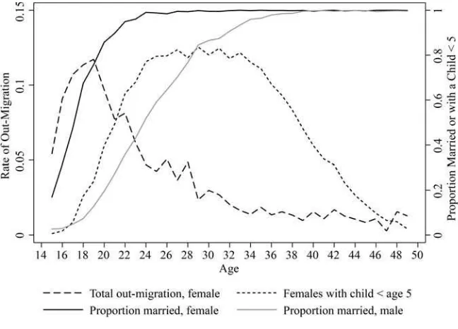
We restrict the sample to women age 25–44 and men age 30–49 in order to focus on men and women who are most likely to be married and have children younger than age fi ve. This restriction serves two purposes. First, these people are most likely to benefi t from the MCH- FP program as adults. Second, it allows us to focus on labor migration rather than marriage migration as most migration for women is for marriage. We do not restrict the sample to people who are married since marriage itself may be endog-enous. To determine the exact age cutoffs, we use data on the entire study site in 1979 to examine the age of marriage for men and women, the percent of women with a child younger than the age of fi ve, and the migration rate for women (Figure 3). The black solid line in Figure 3 shows the percent of women who were married by a given age. It demonstrates that by age 25 almost all women were married. Therefore, we use age 25 as the lower bound in an attempt to exclude migration for marriage. Most of these women also have a child younger than the age of fi ve by age 25. By age 44, women’s fertility is low and the demand for contraceptives is likely quite low. In addition, less than 2 percent of women have a child younger than age fi ve by this age, and less than Figure 3
1 percent migrate (Figure 3). Therefore, we don’t include women after age 44 since the program is unlikely to affect these women.
As for men, Figure 3 (the grey line) demonstrates that men marry later than women and most men are married by the age of 30. Migration rates are very low by age 50 and few men are likely to have children younger than the age of fi ve at that age, so we focus on men aged 30–49.16 As a falsi
fi cation test, we also examine a group of men aged 19–22 who are less likely than the 30–49 year old males to benefi t from the MCH- FP program as parents, and yet were still too old to receive health services from the program as children.17 It is possible that some people in the sample age ranges
were affected by exposure to people who did benefi t from the program as children. For example, the presence of fewer, healthier young people entering the labor market could have potentially affected labor market conditions facing people in our sample. To help limit these possibilities, we end our analysis in 1991.18
D. Dependent Variables and Analytic Data Set
We use the DSS data to construct an individual- year- level longitudinal data set cover-ing the years 1979–91 to represent the fl ow and stock of out- migrants. The data set includes all people who lived in the study area (that is, all people in the DSS) in the fi rst year of the program, 1978. We examine the effect of the program on the average annual fl ow and stock of out- migrants over the three study time periods.
To study the fl ow of out- migrants we limit the data set to include only those who are in the sample age ranges in the current observation year (that is, females 25–44, males 30–49, and males 19–22) in order to examine the effect of the program on people of similar ages over time (that is, people enter or exit the sample based on their age in the current year). The analysis on the fl ow of out- migrants provides information on the share of people in the sample age ranges present in the study area in a given year who migrate out of Matlab that year.
To study the stock of out- migrants, we create a panel data set and follow a cohort of people that was in the sample age ranges in 1978. The analysis on the stock of out- migrants provides information on the share of individuals in the age cohort that was present in the study area at the beginning of the program but lives outside the study area in a given year.
The construction of the dependent variable differs for out- migration fl ow and stock. For out- migration fl ow, the binary indicator variable takes on the value one if a person
16. We do not display data on the percent of men with a child younger than age fi ve because it is missing for many men due to the diffi culty of linking children to their fathers in the data. However, using the data that do exist shows that less than 4 percent of men aged 50 have a child and there is a drop in the percent around age 49.
17. While 19–22- year- olds could move with their families, the vast majority of their moves, unlike those of younger or older men or same- age women, were solo moves for employment or schooling. Results are not sensitive to the exact age cut off.
left the study area that year and lived outside the study area for at least six months, missing if a person migrated out in a prior year and has not returned, and is zero if the person remained in the study area throughout the year. For the stock of out- migrants the binary variable is one in a given year if an individual is an out- migrant (to any des-tination) and zero if the person is not an out- migrant. If a person died, all subsequent observations for both the fl ow and stock are set to missing.19
The fl ow of total out- migrants is disaggregated into domestic, international, or un-known destination. The out- migration variable by destination is made in a similar manner to total out- migration, except that it takes on the value one if the person mi-grated out to the specifi c destination (for example a domestic location) and is assigned zero if they migrated out to a different or unknown destination (such as an interna-tional or unknown destination). Therefore, the sum of the yearly out- migration fl ow rates or regression results for each destination equals the rate or regression results of total out- migration fl ow (migration to any destination).20 In the regression analysis, we
present the program impact on the total fl ow of out- migrants, as well as domestic and international out- migration, to determine whether effects differ by destination.
E. Trends in Rates of Out- Migrant Flow by Destination and Religion
In order to highlight the trends in migration by destination and the distinct pattern of migration of the majority Muslim and minority Hindu populations, Table 1 presents the yearly rates of out- migrant fl ow by religion and destination averaged over the three main time periods. The total out- migration rate is the sum of migration to domestic, international, and unknown destinations. Overall, the total out- migration rate is fairly high at 2 to 3 percent per year in the study area. The vast majority of out- migration was to domestic destinations, and more than 90 percent of domestic out- migration was by Muslims. By contrast, the international fl ow of out- migrants was low and domi-nated by the Hindu minority. For example, between 1979 and 1981, the average rate of international out- migration was less than 0.25 percent, and Hindus, who represent less than 15 percent of the study population, accounted for 90 percent of international moves for women 25–44 and approximately 50 percent for men 30–49. The interna-tional out- migration rate did rise over time to 0.41 percent per year for women and 1.13 percent per year for men during the 1989–91 period.
The domination of international migration by the Hindu population is partially a historical legacy of the partition of India when Bangladesh (then East Pakistan) was created as a Muslim majority state with a sizable Hindu minority. As a result, during the study period Hindus in rural Bangladesh, often economically marginal to start with, continued to migrate (Chowdhury 2009). The general rise in international mi-gration over time is due to an increase in guest worker mimi-gration to the Middle East and Southeast Asia in the 1980s. The international migration rate is still relatively low compared to later in the 1990s because the increase in guest worker migration continued throughout the 1990s and 2000s.
19. Deaths that occur after someone migrates out of the study area are unknown and not recorded. However, death rates are relatively low for people in the sample age ranges as they are still young.
T
he
J
ourna
l of H
um
an Re
sourc
es
Table 1
Rate of Out- Migrant Flow by Destination, Time Period, and Religion (in Percentages)
1979–81 1983–88 1989–91
All Muslim Hindu All Muslim Hindu All Muslim Hindu
Panel A: Females 25–44
Total 1.90 1.62 0.30 2.54 2.10 0.44 3.01 2.39 0.62
Domestic 1.72 1.56 0.17 2.30 2.08 0.22 2.52 2.31 0.21
International 0.14 0.02 0.12 0.24 0.02 0.22 0.41 0.01 0.40
Unknown 0.04 0.04 0.01 0.00 0.00 0.00 0.08 0.07 0.01
Panel B: Males 30–49
Total 2.51 2.18 0.33 2.77 2.31 0.46 3.18 2.54 0.64
Domestic 2.18 1.98 0.20 2.19 1.98 0.21 2.00 1.83 0.17
International 0.23 0.11 0.12 0.58 0.33 0.25 1.13 0.66 0.47
Unknown 0.10 0.09 0.01 0.00 0.00 0.00 0.05 0.05 0.00
Because the pattern and the reasons for domestic and international migration may differ, we present results for migration to all destinations and separately for domestic and international migration. Further, to account for the differences in domestic and in-ternational migration patterns between Hindus and Muslims, we include a control for being Hindu and allow the year fi xed- effects to vary by religion. We also drop Hindus from the sample as a robustness check.
F. Trends in Rates of Out- Migrant Flow and Stock by Treatment Status
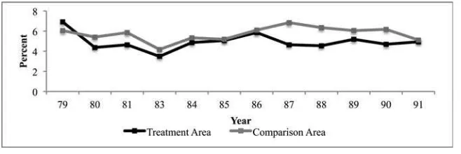
Figures 4a and b present trends in the yearly rate of out- migrant fl ow (left axis) and stock (right axis) from 1979–1991 for women aged 25–44 and men aged 30–49. Data for 1982 are not included due to the data issues discussed in Section IIIA. The dis-played trends in the fl ow of out- migrants demonstrate that, in the early part of the program (1979–81), the rates of out- migration were fairly similar between the treat-ment and comparison areas for both men and women. After 1981, however, there was a large increase in the rate of out- migration in the comparison area for women and men. There was a similar increase in out- migration across Bangladesh during this time period (Afsar 2003). However, the treatment area did not experience the same increase in the rate of out- migration as did the comparison area. The difference in the rate of out- migrant fl ow between the two areas narrows after 1988. The trends in rate of out- migrant stock takes into account the fl ow of return migrants, which suggests that more people from the comparison area remained outside the study area, especially after 1983.
In Figure 4c, we display the fl ow of out- migration for men aged 19–22, the falsifi ca-tion group that is less likely to benefi t from the program as adults. Migration rates for this group are similar between the treatment and comparison area until 1986. Starting in 1987, the migration rates between the treatment and comparison area begin to differ for these men. The difference in the migration rates between the two areas is likely a result of Meghna- Dhonnogoda embankment and highlights the need to control for the embankment in all the analyses.
IV. Estimation Strategy
A. Quasi- random Program DesignFigure 4c
Trends in Rates of Total Out- Migrant Flow—Males 19–22
Note to all frames: 1982 data not included due to issues with the data for that year. Figure 4a
Trends in Rates of Total Out- Migrant Flow and Stock—Females 25–44
Figure 4b
also shows that most household pre- intervention characteristics are balanced, and that levels of cognitive functioning were similar between the treatment and comparison area in 1996 for those who did not receive direct health services from the program.
We use the 1974 census data to test whether individual, household, and household- head characteristics are similar between treatment and comparison areas prior to the program. The sample includes females age 25–44 and males 30–49 in the 1974 cen-sus. We look at individuals in our sample age ranges in 1974 to determine whether or not the types of households that the adults in the relevant age groups come from are balanced prior to the program. Results are similar if we examine the 1974 char-acteristics for our actual samples used in the paper. Table 2 presents means for the treatment and comparison group separately and the differences in means between the two groups.21 We report the statistical signi
fi cance of the differences in means between the treatment and comparison areas, and the normalized differences in means (differ-ence in the means divided by the standard deviation of the mean for the sample). The normalized difference provides an indication of the size of the differences in means because even small differences in means can be statistically signifi cant with large sample sizes (Imbens and Wooldridge 2009). Normalized differences bigger than 0.25 standard deviations are generally thought to be substantial.
Table 2 highlights the fact that the differences in means for the treatment and com-parison areas in 1974 are statistically insignifi cant at the 5 percent level for all vari-ables except years of education, religion, the household’s drinking water source, and the household’s number of rooms per capita. However, the normalized differences are small and less than 0.14 for all variables except religion and drinking water sources. The percent of Hindus and households with access to tube well water is higher in the treatment area than the comparison area by 10 and 17 percent respectively, and the normalized differences are greater than 0.25. The large difference in access to tube well water is a result of a government program22 so does not necessarily refl ect other
unobservable differences between the treatment and comparison areas that could be correlated with a person’s propensity to migrate (such as household income or house-hold’s concern about health).
These fi ndings, together with results of previous studies on fertility and mortality, strongly suggest that the two areas had very similar observable characteristics with the exception of religion and access to tube well water. To help control for biases created by any differences in the baseline characteristics between the treatment and comparison areas, we control for all 1974 baseline variables in Table 2 interacted with time period dummies for the three periods of interest (1979–81, 1983–88, 1989–91), except for marital status and religion.23 We do not control for marital status because it
may be endogenous but report it in Table 2 to highlight that it is balanced in 1974. As
21. Results are presented for men and women together but results by gender are similar to the population as a whole.
22. In 1968 the government of Bangladesh (then East Pakistan) set a goal of installing one tube well for every 200 people. With the support of the United Nations Children Fund, by 1978 over 300,000 tube wells had been sunk, about one for every 250 rural inhabitants (Black 1986).
T
he
J
ourna
l of H
um
an Re
sourc
es
Treatment Area Comparison Area Difference in Means
Mean SE Observations Mean SE Observations Mean T- stat Mean/SD
Individual Characteristics
Years of education females 0.94 (0.06) 9,246 0.75 (0.04) 9,192 0.20 2.79 0.11 Years of education males 2.87 (0.11) 7,918 2.43 (0.08) 7,754 0.43 3.12 0.13
Married 0.94 (0.00) 17,237 0.93 (0.00) 17,002 –0.00 1.12 0.01
Muslim (=1) 0.78 (0.04) 17,237 0.88 (0.03) 17,002 –0.10 –1.98 –0.26
Household Characteristics
Family size 6.88 (0.06) 17,215 6.77 (0.05) 16,979 0.11 1.50 0.04
Percent of household members aged:
0–4 0.17 (0.00) 17,215 0.17 (0.00) 16,979 0.00 0.16 0.00
5–9 0.17 (0.00) 17,215 0.17 (0.00) 16,979 0.00 0.23 0.01
10–15 0.17 (0.00) 17,215 0.17 (0.00) 16,979 –0.00 –1.22 –0.02
Owns a lamp (=1) 0.63 (0.02) 17,204 0.60 (0.01) 16,966 0.03 1.07 0.06 Owns a watch (=1) 0.14 (0.01) 17,204 0.13 (0.01) 16,966 0.01 1.14 0.04 Owns a radio (=1) 0.08 (0.01) 17,204 0.08 (0.00) 16,966 0.01 0.77 0.02 Wall tin/tinmix (=1) 0.30 (0.01) 17,053 0.30 (0.01) 16,786 0.00 –0.09 0.00 Tin roof (=1) 0.79 (0.01) 17,065 0.80 (0.01) 16,788 –0.01 –0.45 –0.02
Latrine (=1) 0.79 (0.02) 17,201 0.83 (0.03) 16,964 –0.04 –1.10 –0.09
Number of rooms per capita 0.20 (0.00) 17,215 0.20 (0.00) 16,979 0.00 2.29 0.05
Number of cows 1.30 (0.06) 17,199 1.18 (0.04) 16,966 0.12 1.64 0.07
Number of boats 0.62 (0.03) 17,202 0.64 (0.02) 16,966 –0.01 –0.31 –0.02 Drinking water:
Tube well (=1) 0.34 (0.04) 17,204 0.17 (0.02) 16,955 0.17 4.27 0.40
Tank (=1) 0.37 (0.04) 17,204 0.32 (0.03) 16,955 0.05 1.09 0.11
Other (=1) 0.28 (0.05) 17,204 0.51 (0.04) 16,955 –0.23 –3.83 –0.46
Household Head Characteristics
Age 45.2 (0.24) 17,200 44.7 (0.17) 16,963 0.45 1.54 0.04
Works in agriculture (=1) 0.58 (0.02) 17,207 0.55 (0.02) 16,968 0.03 0.90 0.06 Works in fi shing (=1) 0.08 (0.02) 17,207 0.10 (0.01) 16,968 –0.02 –0.86 –0.07 Spouse’s age 34.4 (0.20) 15,703 34.2 (0.16) 15,557 0.25 0.96 0.03
discussed in Section IIIE, we control for religion with Hindu- year fi xed effects interac-tions and as a robustness check exclude Hindus from the analysis.
B. Identifi cation Strategy
To identify the treatment effect of the MCH- FP program on out- migration, we exploit variation in program implementation between the treatment and comparison areas and estimate intent- to- treat effects. In addition, we take advantage of the phasing- in of the interventions over time within the treatment area to examine the effect of the program for three main time periods: (1) the 1979–81 period when family planning and some basic maternal health interventions were introduced; (2) the 1982–88 period when most child health interventions were introduced; and (3) the 1989–91 period when many of the program interventions became available through government services in the comparison area. Because data for 1982 is not included in the analysis due to data issues, the tables indicate the middle time period is from 1983–88.
Due to data restrictions, it is not possible to control for preprogram differences in migration rates. Instead, we examine both single and double difference estimates of the treatment effect, where we use the 1979–81 period, when only some of the program interventions had been introduced, as the baseline period for the double dif-ference model. To the extent there are already program effects in the 1979–81 period, the double difference model will underestimate the program effect.
C. Empirical Specifi cation
Hindu- year fi xed effects interactions; 1974 information on a person’s years of educa-tion attained; all 1974 household and household- head characteristics shown in Table 2 interacted with the three time periods (“baseline- period” controls); and preprogram village fi xed effects to account for nontime- varying differences between villages. When preprogram village fi xed effects are included, β1 drops out of the model since this effect is absorbed by the preprogram village fi xed effects, making the single- and double- difference results similar. The error term is clustered at the village level to account for the likely intracluster and serial correlation as well as heteroskedasticity inherent in the linear probability model.
The βs are the single- difference estimates of the program effect. For the out- migration fl ow models, they indicate the average difference in the yearly probability of migration out of the study site between the treatment and comparison area for the three time periods. When multiplied by 100 the βs represent percentage point differences in the fl ow of out- migrants between the treatment and comparison area. In contrast, for models examining the stock of out- migration, when the βs are multiplied by 100 they indicate the percentage point difference between the treatment and comparison area of individuals present in the study area in the fi rst year of the program that are living outside the study area. For both models, the βs can be used to determine the double- difference estimate in the latter two periods by subtracting β1from β2or β3.
V. Program Impacts
A. Program Effects on Flow of Out- MigrantsThe treatment effects on out- migration fl ow to all destinations as well as to domes-tic and international destinations are presented in Table 3 for females aged 25–44 and Table 4 for men aged 30–49.24,25 All regressions include observation- year and
age- fi xed effects, a control for being Hindu, and controls for living in an erosion or Meghna village at baseline. We include additional controls across Columns 2–4 to control for any differences between the treatment and comparison areas. The embank-ment controls are included in Column 2 and should reduce the program effects. The single- difference program estimates are presented in Panel A. It is diffi cult to compare the magnitude of the coeffi cients across males and females or time periods because the base migration rates differ. Therefore, in Panel B we report the percent change in the probability of migration relative to the comparison group mean for the time period of interest. The p- value from the double- difference estimator is presented in Panel C of Tables 3 and 4.
24. We also investigated the heterogeneous effects of the program between those with some and no educa-tion, and those who own or do not own land. We found no signifi cant differences in the probability of out- migration between these two groups.
Ba
rha
m
a
nd K
uhn
1003
Total Domestic International
1 2 3 4 5 6 7
Panel A: Single- difference estimates
1979–81 –0.0016 –0.0029 –0.0023 –0.0024 –0.0007 –0.0016
(0.0021) (0.0018)+ (0.0017) (0.0017) (0.0017) (0.0009)+
1983–88 –0.0068 –0.0047 –0.0047 –0.0026 –0.0041 –0.0056 0.0009
(0.0016)** (0.0013)** (0.0013)** (0.0019) (0.0012)** (0.0012)** (0.0006)
1989–91 –0.0016 –0.0031 –0.0028 –0.0009 –0.0031 –0.0028 0.0003
(0.0020) (0.0019)+ (0.0020) (0.0024) (0.0020) (0.0018) (0.0007) Panel B: Single- differences—percent changes
1979–81 –8 –14 –11 –12 –4 –89
1983–88 –22 –15 –15 –8 –14 –19 48
1989–91 –5 –10 –9 –3 –10 –10 8
Panel C: P- value for Double- Difference Estimates
1983–88 0.062 0.341 0.190 0.337 0.005 0.012
1991–89 0.991 0.931 0.827 0.766 0.328 0.074
Embankment controls N Y Y Y Y Y Y
Baseline- period controls N N Y Y Y Y Y
Village fi xed effects N N N Y N N N
Drop erosion area N N N N Y N N
Adjusted R2 0.01 0.01 0.02 0.02 0.01 0.02 0.02
Observations 232,906 232,906 232,906 232,906 226,056 232,906 232,906
T
he
J
ourna
l of H
um
an Re
sourc
es
Table 4
Treatment Effects on Annual Flow of Out- Migrants—Males 30–49 in Current Year
Total Domestic International
1 2 3 4 5 6 7
Panel A: Single- Difference Estimates
1979–81 0.0003 –0.0007 –0.0011 –0.0015 0.0004 –0.0017
(0.0024) (0.0024) (0.0022) (0.0022) (0.0018) (0.0009)+
1983–88 –0.0079 –0.0058 –0.0056 –0.0049 –0.0052 –0.0059 0.0003
(0.0020)** (0.0019)** (0.0019)** (0.0026)+ (0.0018)** (0.0015)** (0.0010)
1989–91 –0.0029 –0.0033 –0.0033 –0.0023 –0.0032 –0.0040 0.0010
(0.0025) (0.0026) (0.0028) (0.0030) (0.0028) (0.0020)* (0.0015) Panel B: Single- Difference Estimates—Percent Change
1979–81 1 –3 –4 –6 2 –63
1983–88 –23 –17 –17 –14 –16 –21 6
1989–91 –8 –9 –9 –7 –10 –16 10
Panel C: P- value for Double- Difference Estimates
1983–88 0.009 0.047 0.074 0.138 0.002 0.152
1991–89 0.296 0.393 0.452 0.571 0.050 0.119
Embankment controls N Y Y Y Y Y Y
Baseline- period controls N N Y Y Y Y Y
Village fi xed effects N N N Y N N N
Drop erosion area N N N N Y N N
Adjusted R2 0.01 0.01 0.01 0.01 0.01 0.01 0.01
Observations 177,335 177,335 177,335 177,335 172,634 177,335 177,335
1. Total Out- Migration.
We fi rst examine if there is a difference in the single- difference estimates of the prob-ability of total out- migration between the treatment and comparison area during the 1979–81 period (Row 1979–81 of Panels A and B). Tables 3 and 4 demonstrate that there are no statistically signifi cant differences at the 5 percent level or lower for either females or males for any of the specifi cations (Columns 1–3). The difference in the probability of out- migration is lower in the treatment than the comparison area by 11 percent for women and 4 percent for men with inclusion of embankment and baseline controls (Specifi cation 3 Panel B).
During the 1983–88 period, the single- difference estimates of the probability of mi-gration between the experimental groups declines for both sexes between Columns 1 and 2 in Tables 3 and 4 with the introduction of the embankment controls, as expected. Column 2 indicates that with the inclusion of the embankment controls the difference in the probability of total out- migration between the two areas was –0.0047 for females and –0.0058 for men and is statistically signifi cant at the 1 percent level. As shown in Panel B, these reductions represent a 15 and 17 percent lower out- migration rate in the treatment compared to the comparison area for women and men, respectively. The pro-gram effects are the same when the baseline- period controls are included in Column 3 and still statistically signifi cant different at the 1 percent level. The similarity in results with and without the inclusion of the baseline- period controls provides some evidence that any differences in preprogram characteristics, such as religion and access to tube well water, are not biasing the results. The introduction of village fi xed effects in Column 4 leads the program effect to decline to 8 percent for women and 14 percent for men and is no longer statistically signifi cant for women and is signifi cant at the 10 percent level for men.26 The reduction in the program effect between Speci
fi cations 3 and 4 is a result of the village fi xed effects accounting for the difference in migration rates between the treatment and comparison areas during the 1979–81 period.
The double- difference program effect for total out- migration during the 1983–88 pe-riod is smaller than the single- difference effect due to the differences between the groups during the 1979–81 period. The double- difference point estimates are not reported but, based on calculations using single- difference estimates from Column 3, for women it is –0.0024 and for men –0.0045, though the effects are no longer statistically signifi cant for women and marginally signifi cant, at the 10 percent level, for men (Panel C).
By the 1989–91 period, program effects are lower than during the 1983–88 period for both women and men and are no longer statistically signifi cant for either the single or double difference estimator in Column 3. It is not surprising that the point estimates are lower because there were improvements in the supply of government services in the comparison area during the 1989–91 time period.
2. Domestic and International Out- Migration
We disaggregate total migration into domestic and international out- migration to ex-amine if program effects vary by destination (Columns 6 and 7 of Table 3 for women
and Table 4 for men).In the fi rst period, 1979–81, the difference in the probability of domestic out- migration between the treatment and comparison areas is small. As shown in Panel B, it is 4 percent lower for women, and 2 percent higher for men and not statistically signifi cant. Due to the limited difference in rates of domestic migration between treatment and comparison area in the 1979–81 period, double- differences re-sults for domestic out- migration are similar to the single- difference rere-sults in the later two periods. The difference in the results between the total and domestic out- migration is driven by international migration. The international migration rate is lower in the treatment area than the comparison area, and the difference is marginally statistically signifi cant (at the 10 percent level). International- migration rates were especially low during this period so results should be interpreted with care.
During the 1982–88 period, the single- difference program effect for domestic out- migration is higher than for total out- migration; the probability of domestic out- migration is lower in the treatment than the comparison area by 19 percent for women and 21 percent for men and statistically signifi cant at the 1 percent level. The double- difference program effect for domestic out- migration is also signifi cantly different at the 1 percent level for women and men (Panel C). The magnitude of the effect for women is –0.0049 (–17 percent) and for men –0.0063 (–22 percent). For interna-tional migration, the single- difference program effect is not statistically signifi cant for women or men. Double- difference effects for international out- migrants are positive and statistically signifi cant at the 5 percent level for women but the size and signifi -cance of the effect is being driven by the difference in international out- migration rates between the treatment and comparison areas during the 1979–81 period.
During the 1989–91 period, single difference program effects declined from the earlier period for domestic out- migration to 10 percent for women and 16 percent for men. They are no longer statistically signifi cant for women but are for men at the 10 percent level. There are no statistically signifi cant program effects during this period on international migration.
B. Robustness and Falsifi cation Checks on the Flow of Out- Migrants
We perform a number of robustness and falsifi cation checks on the fl ow of out- migration based on specifi cation 3 of Tables 3 and 4, some of which are presented in Tables 2–4 of the online Appendix and can be found at http://jhr.uwpress.org/. First, because the embankment project led to the destruction of the erosion villages, we excluded from the sample any individual who lived in an erosion village since 1977 and report the results in Column 5 of Tables 3 and 4. The results are very similar to those reported in Column 3, which is not surprising since the embankment controls accounted for the higher out- migration from the erosion villages.
com-parison area. The double- difference program effects are slightly smaller but still sta-tistically signifi cant at the 1 percent level for women and the 5 percent level for men. Third, the propensity of someone to return to the study area after migrating away could be different between the treatment and comparison area prior to the program, bi-asing our results on the fl ow of out- migrants. To account for this possibility, for people who have multiple out- migration events during the study period due to return migra-tion, we restrict the sample to include only a person’s fi rst out- migration event. Again, we fi nd a similar pattern of results, with a statistically signifi cant single- difference effect in the 1983–88 period of –13 percent for women and men for migration to any destination and approximately –18 percent for migration to domestic locations (online Appendix Tables 2 and 3, Columns 3 and 4).
Fourth, it is possible that the program affected the composition of people who aged into the sample if it led to differential out- migration patterns of these individuals be-fore we observe them in the sample, thus potentially biasing the results. To control for this possibility, we examine the program effects on a cohort of people in the sample age ranges in 1978 (mimicking the stock sample) rather than allowing people to age in and out of the sample over the time period. Explicitly, we use panel data to follow a cohort of females aged 25–44 and males aged 30–49 in 1978 (online Appendix Tables 2 and 3, Columns 5 and 6). The pattern and magnitude of results is similar. During the 1983–88 period, the single- difference results show a reduction in total out- migration due to the program of 14 percent for women and 18 percent for men.
Fifth, we drop anyone for whom there is no 1974 census data since missing baseline control information was fi lled in with experimental area means. This excludes people who were not present at the time of the 1974 census or moved into the area between the census and the start of the program (online Appendix Tables 2 and 3, Columns 7 and 8). Again, we fi nd results similar to the main results.
Finally, as a falsifi cation test, we examine the effect of the program on men aged 19–22 (online Appendix Table 4). We expect there to be a lower or different impact on this group as most were not married and had no children so would not directly benefi t from the program as adults. However, they may have benefi ted as children from the program due to having fewer (and perhaps healthier) younger siblings. There are no statistically signifi cant program effects for any of the three time periods, and the point estimates for the 1983–88 period are positive rather than negative. This provides some further confi dence that the reduction in total and domestic out- migration fl ows due to the program during the 1983–88 time period for females aged 25–45 and males aged 30–49 are not likely a result of unobservable, time- varying characteristics.
C. Program Effects on Migrant Stock
T
he
J
ourna
l of H
um
an Re
sourc
es
Table 5
Treatment Effect on the Annual Stock of Total Out- Migrants—By Cohort (Indicated by Age in 1978)
Females Males
25–44 1
35–44 2
25–34 3
30–49 5
40–49 6
30–39 7
Panel A: Single- Difference Estimates
1979–81 –0.0017 –0.0025 –0.0012 –0.0019 –0.0024 –0.0020
(0.0021) (0.0022) (0.0030) (0.0028) (0.0031) (0.0036)
1983–88 –0.0136 –0.0138 –0.0136 –0.0102 –0.0113 –0.0104
(0.0053)* (0.0056)* (0.0073)+ (0.0073) (0.0078) (0.0094)
1989–91 –0.0216 –0.0144 –0.0289 –0.0206 –0.0141 –0.0283
(0.0075)** (0.0079)+ (0.0099)** (0.0102)* (0.0112) (0.0125)* Panel B: Single- Difference Estimates—Percent Change
1979–81 –10 –22 –5 –8 –15 –7
1983–88 –19 –25 –15 –10 –15 –8
1989–91 –19 –16 –21 –13 –12 –15
Panel C: P- value for Double- Difference Estimates
1983–88 0.008 0.018 0.040 0.173 0.178 0.286
1991–89 0.004 0.104 0.002 0.047 0.257 0.023
Adjusted R2 0.06 0.06 0.06 0.06 0.06 0.06
Observations 214,072 102,305 111,767 170,612 84,217 86,395
women and men, and include controls used in Specifi cation 3 of the out- migrant fl ow analysis.
For females aged 25–44 in 1978 (Column 1), there is no statistically signifi cant program effect during the 1979–81 period. However, by the 1983–88 period the stock of out- migrants was 1.36 percentage points (Panel A Column 1) lower in the treatment than in the comparison area, and the difference is statically signifi cant at the 1 percent level. Relative to the comparison group mean for the 1983–88 time period, this is a reduction in the stock of out- migrants (Panel B Column 1) of 19 percent for the 25–44 year cohort. By the 1989–91 period, the difference in the stock of out- migrants be-tween the treatment and the comparison area was larger at 2.16 percentage points, but this still represents a program effect of 19 percent. The double- difference results for the latter two time periods are smaller but the statistical signifi cance is the same as for the single- difference results. Finally, the program had effects on both of the 10- year cohorts. By the 1989–91 period, the stock of migrants was 16 percent lower for the 35–44- year- old cohort and 21 percent lower for the 25–34- year- old cohort (Columns 2 and 3 of Panel B).
For males, there are no statistically signifi cant program effects until the 1989–91 period. By this time period, the stock of out- migrants was 2.06 percentage points (Panel A Column 5) lower in the treatment than in the comparison area for those aged 30–49 in 1978, and the difference is statically signifi cant at the 5 percent level. This difference represents a 13 percent decline relative to the comparison group mean for the time period. The decline in percent terms is between 12–15 percent for the two 10- year cohorts, but it is only statistically signifi cant at the 5 percent level for the younger cohort aged 30–39 in 1978.
As a robustness check, in Table 4 of the online Appendix we include a fourth time period, from 1992–95, to allow more time for return migration. Results in Panel B show the magnitude of the program effects in the 1992–95 period are similar to those in the 1989–91 period, indicating that the stock of migrants did not substantially change between the 1989–91 and 1992–95 periods.
These results highlight that, even in a context with substantial return migration, the differences in the fl ow of migration brought about by the benefi t program persist in driving longer- term changes in the stock of out- migrants in the area.
VI. Conclusion
This paper takes advantage of a highly effective health and family planning intervention, The Matlab Maternal and Child Health and Family Planning, and provides new evidence on the impact of local benefi t programs on out- migration. The program was quasi- randomly assigned in geographically contiguous areas. One important benefi t of this block design is that our estimates are not likely to be biased by the large potential spillovers associated with the childhood vaccines provided by the program. We further take advantage of individual- level migration data to precisely estimate out- migration fl ows and stock and to address potential confounding factors.