Achievement
Results from the Moving to Opportunity
Experiment
Lisa Sanbonmatsu
Jeffrey R. Kling
Greg J. Duncan
Jeanne Brooks-Gunn
a b s t r a c t
Families originally living in public housing were assigned housing vouchers by lottery, encouraging moves to neighborhoods with lower poverty rates. Although we had hypothesized that reading and math test scores would be higher among children in families offered vouchers (with larger effects among younger children), the results show no significant effects on test scores for any age group among more than 5,000 children aged six to 20 in
Lisa Sanbonmatsu is a Postdoctoral Fellow at the National Bureau of Economic Research (NBER). Jeffrey R. Kling is a Senior Fellow in Economics at the Brookings Institution and a Faculty Research Fellow at NBER. Greg J. Duncan is the Edwina S. Tarry Professor of Human Development and Social Policy at Northwestern University. Jeanne Brooks-Gunn is the Virginia and Leonard Marx Professor of Child Development and Education at Teachers College, Columbia University. The authors thank the U.S. Department of Housing and Urban Development, the National Institute of Child Health and Human Development (NICHD), the National Institute of Mental Health (R01-HD40404 and R01-HD40444), the National Science Foundation (SBE-9876337 and BCS-0091854), the Robert Wood Johnson Foundation, the Russell Sage Foundation, the Smith Richardson Foundation, the MacArthur Foundation, the W. T. Grant Foundation, and the Spencer Foundation for funding the interim MTO evaluation and our research. Additional support was provided by grants to Princeton University from the Robert Wood Johnson Foundation and from the NICHD (5P30-HD32030 for the Office of Population Research) and by the Princeton Industrial Relations Section, the Bendheim-Thoman Center for Research on Child Wellbeing, the Princeton Center for Health and Wellbeing, and the National Bureau of Economic Research (NBER). The authors are grateful to Todd Richardson and Mark Shroder of HUD, to Judie Feins, Barbara Goodson, Robin Jacob, Stephen Kennedy, and Larry Orr of Abt Associates, to our collaborators Alessandra Del Conte Dickovick, Jane Garrison, Lawrence Katz, Jeffrey Liebman, Tama Leventhal, Jens Ludwig, and to numerous colleagues for their suggestions. The data used in this article are available from the U.S. Department of Housing and Urban Development (HUD) to researchers who meet HUD’s data confiden-tiality requirements described at http://www.huduser.org/publications/fairhsg/MTODemData.html. Direct questions about the availability to Lisa Sanbonmatsu, 617-613-1201 <lsanbonm@nber.org> or to HUD’s Todd Richardson, 202-708-3700 ¥5706 <todd_m._richardson@hud.gov>.
[Submitted August 2004; accepted December 2005]
ISSN 022-166X E-ISSN 1548-8004 © 2006 by the Board of Regents of the University of Wisconsin System
2002 who were assessed four to seven years after randomization. Program impacts on school environments were considerably smaller than impacts on neighborhoods, suggesting that achievement-related benefits from improved neighborhood environments alone are small.
I. Introduction
Children educated in large urban school districts in the United States have substantially lower academic performance than children in the nation as a whole.1Children attending schools with high concentrations of poor students fare par-ticularly poorly, facing numerous disadvantages including less-educated parents, low performing schools, and distressed communities outside of school (Lippman, Burns, and McArthur 1996). In an attempt to identify the effects of social context that are dis-tinct from individual and family factors, this paper examines the extent to which changes in residential neighborhood affect children’s academic achievement.
Our analysis utilizes a randomized housing mobility experiment, the Moving to Opportunity (MTO) for Fair Housing demonstration program of the U.S. Department of Housing and Urban Development (HUD), to estimate the causal effects on chil-dren’s educational outcomes of moving out of high-poverty neighborhoods. Through a lottery for housing vouchers among families initially living in public housing, MTO randomly assigned families into three groups. Families in an “experimental” group received housing vouchers eligible for use in low-poverty neighborhoods. Families in a “Section 8” group received traditional housing vouchers without neighborhood restrictions. Families in a control group did not receive either voucher, but were still eligible for public housing.
While family and individual attributes may strongly influence children’s educa-tional outcomes, the experimental design of MTO enables us to isolate the impact of residential neighborhood characteristics on educational outcomes. If neighborhoods influence the quality and learning environment of schools attended, then residential relocation programs such as MTO should improve educational outcomes among chil-dren who experience moves through the program. Neighborhoods also may affect the educational norms, values, and resources in the community outside of school. These community influences may be particularly important for young children who have spent the largest fraction of their lives in new locations, may be more adaptable to a new social environment, and are learning language at a rapid rate (Shonkoff and Phillips 2000). Children not old enough to attend school prior to their families’ MTO enrollment had the opportunity to begin their schooling in a less impoverished neigh-borhood. Both school readiness and school success in the early grades may be impor-tant for later school success and human capital formation (Rouse, Brooks-Gunn, and Sara McLanahan 2005; Slavin, Karweit, and Wasik 1993; Heckman 2000).
In the analysis that follows, we focus on estimating the magnitude of impacts on educational outcomes and evaluating the mechanisms through which neighborhoods may produce them. In addition to assessing the test scores and behavioral gains over-all, we test the hypothesis that younger children would experience greater gains than older children. We also investigate the possibility of differential effects based on demographic characteristics including gender, race, and ethnicity, and educational risk factors. Furthermore, using school address histories and data on school charac-teristics (including self-reports on school climate), we analyze the extent to which moves out of high-poverty neighborhoods imply moves to higher-quality schools—a principal mechanism through which residential mobility programs can affect educational outcomes.
In Section II, we review existing literature on the association between neighbor-hoods and educational outcomes. In Section III, we present the details of the MTO program. Section IV discusses our data sources, and Section V outlines our econo-metric approach. Sections VI and VII present our results and Section VIII concludes.
II. Existing Literature
The impact of neighborhoods on children’s outcomes is subject to wide debate.2From a theoretical perspective, residential mobility and the sorting of individuals into neighborhoods is a key factor in the production of human capital (Benabou 1993; Fernandez 2003). Some researchers argue that early childhood envi-ronments, in combination with individual attributes and family background, influence subsequent outcomes much more than environmental conditions in later childhood or adolescence (Bouchard 1997; Duncan et al. 1998; Shonkoff and Phillips 2000). Developmental theory and studies of school failure suggest that arguments concern-ing the importance of early influences may be particularly relevant for educational achievement (Slavin, Karweit, and Wasik 1993). Others believe that disadvantaged neighborhoods may have adverse effects on adolescent development by depriving youth of positive peer influences, adults who provide role models and actively moni-tor neighborhood events, and school, community, and healthcare resources, as well as by exposing them to violence (Sampson, Raudenbush, and Earls 1997).
In contrast to theories about the deleterious effects of disadvantaged neighbor-hoods, “relative deprivation” models argue that poor families may actually fare better in low-income neighborhoods; in high-income neighborhoods, these families may face discrimination or may experience resentment. These models predict that children in low-income families living in high-income neighborhoods will exhibit worse out-comes, including low educational attainment, behavioral problems, and diminished mental health (Wood 1989; Marsh and Parker 1984; Collins 1996).
The bulk of the empirical research to date studying neighborhood effects and youth educational outcomes uses nonexperimental data, typically linking developmental
studies of children to Census data on local area characteristics. For example, studies focusing on the reading achievement and vocabulary outcomes of five- to six-year-olds have generally found that more affluent neighborhoods are associated with higher achievement in comparison with middle income neighborhoods, even after control-ling for family sociodemographic characteristics (Chase-Lansdale and Gordon 1996; Chase-Lansdale et al. 1997; Duncan, Brooks-Gunn, and Klebanov 1994; Kohen et al. 2002). Researchers focusing on older youth have found that higher neighborhood socioeconomic status is associated with higher combined reading and math scores (Halpern-Felsher et al. 1997; Ainsworth 2002) and greater likelihood of high school graduation (Aaronson 1998).3While these nonexperimental studies are suggestive, the causal link between neighborhoods and educational outcomes is not clear; observa-tionally equivalent families selecting to live in different neighborhoods may be differ-ent on unobserved characteristics—characteristics that also may influence educational outcomes for their children. Duncan, Boisjoly, and Harris (2001) and Solon, Page, and Duncan (2000) show that correlations between neighboring children in their achieve-ment scores and subsequent educational attainachieve-ment are small once family background is controlled for, suggesting only a limited role for neighborhood factors.
Researchers have attempted to handle concerns about unobservable differences between individuals living in different neighborhoods by using the quasi-experiment of court-ordered remedial programs, in which federal courts have required HUD to provide funding for rental assistance and housing counseling services in order to reduce racial segregation in publicly assisted housing. In an influential study, Rosenbaum (1995) argued that in Chicago’s Gautreaux program, residential location was essentially determined by quasi-random waitlist ordering, so that families who moved to suburban locations were comparable to those who moved to other in-city locations. He found that children in suburban neighborhoods had higher satisfaction with teachers and had better attitudes about school, and that high school dropout rates were much lower for suburban children—5 percent compared with 20 percent among those in city neighborhoods. Despite the influence of the Gautreaux study, the sample sizes are small and the response rates are low, allowing for the possibility of substantial bias.4
In a more recent study of children moving out of public housing in Chicago due to Hope VI demolitions, Jacob (2004) found no effect on children’s test scores, and found only small changes in neighborhood circumstances despite departure from pub-lic housing. Currie and Yelowitz (2000) found that children in pubpub-lic housing projects were less likely to be held back in school than children in similarly poor families with-out access to public housing and speculate that this resulted from public housing pro-viding better living conditions than these families would have had in the absence of the public housing.
The MTO research platform addresses the selection problem using a randomized design described in detail in Section III. Early MTO work based on about 350
3. For reviews of the literature, see Jencks and Mayer (1990); Brooks-Gunn, Duncan, and Aber (1997); Furstenberg et al. (1999); and Leventhal and Brooks-Gunn (2000).
Baltimore children aged five to 12 found large changes in neighborhood circum-stances for the experimental group relative to the control group and positive effects on reading and math test scores over the first four years after random assignment (Ludwig, Ladd, and Duncan 2001). A study of 168 children aged six to ten at the MTO site in New York did not find effects on test scores for the experimental versus control group overall after three years—although it did find positive effects on test scores for a sample of male youth (Leventhal and Brooks-Gunn 2004).
While the experiment cannot provide a direct method for distinguishing between different mechanisms through which neighborhoods affect children, it can provide more precise estimates of the impact of neighborhoods on educational and other out-comes. This paper uses data on more than 5,000 children aged six to 20 at all five MTO sites, looking at medium-term outcomes four to seven years after random assignment, in order to help solidify our understanding of these effects.
III. The Moving to Opportunity Experiment
The MTO demonstration program was designed to assess the impact of providing families living in subsidized housing with the opportunity to move to neigh-borhoods with lower levels of poverty. Families were recruited for the MTO program from public housing developments in Boston, Baltimore, Chicago, Los Angeles, and New York. HUD primarily targeted developments located in census tracts with 1990 poverty rates of at least 40 percent. Program eligibility requirements included residing in a targeted development, having very low income that met the Section 8 income lim-its of the public housing authority, having a child younger than 18, and being in good standing with the housing authority. From 1994–97, 4,248 eligible families were ran-domly assigned to one of three groups: a control group (n= 1,310), an experimental treatment group (n= 1,729), and a Section 8 treatment group (n= 1,209).5
Each family assigned to the Section 8 group received a housing voucher or certifi-cate that could be used to rent an apartment in the private market, under the standard terms of the federal Section 8 housing program. Each family in the “experimental” group received a similar voucher or certificate, but that could only be used to rent an apartment in a tract with a poverty rate of less than 10 percent (based on 1990 Census data). In order to help the experimental group families comply with this geographic restriction, local nonprofits offered these families mobility counseling.6 The geo-graphic restriction on the experimental group’s voucher applied only for the first year, after which the voucher could be used in any tract. Control group families were not offered housing vouchers, but they could continue to live in public or subsidized hous-ing as long as they remained eligible. Treatment group families who did not use their
5. Families were initially randomly assigned in an 8:3:5 ratio of experimental:Section 8:control group fam-ilies. The initial ratios were chosen to minimize minimum detectable effects of experimental impacts based on forecasted voucher utilization, and were adjusted over time in response to actual utilization.
vouchers within the required time period also could remain in public housing.7 Families residing in public housing or using vouchers to rent apartments in the private market are generally required to pay 30 percent of their adjusted income in rent.
Forty-seven percent of the experimental group families and 59 percent of the Section 8 group families used the program housing voucher to “lease-up,” or move to a new apartment. We refer to the families who moved using a voucher as treatment “compliers.” By randomly assigning families to different voucher groups, the demon-stration was designed to introduce an exogenous source of variation in neighborhood conditions.
IV. Sample and Data
A. Sample and Data Sources
This paper focuses on test score data collected in 2002 for MTO children who were school age or slightly older (aged six to 20 as of December 31, 2001) at the time of interview.8The age range of the sample allows us to examine the impact of neigh-borhoods on educational achievement and to test the hypothesis of stronger effects for younger rather than older children. Most of our information about educational out-comes out-comes from data collected in collaboration with Abt Associates and HUD four to seven years after the families entered the MTO program. One adult and up to two children from each family were selected for this data collection. Interviewers admin-istered a battery of achievement tests to the sample children and interviewed those children who were at least eight years old. The interview asked children about their schools, neighborhoods, friends, health, behavior, and activities. Interviewers also asked adults about their children’s behavior, health, schooling, and activities.
The interview and test score data were collected in two main phases. During the first phase, interviewers attempted to locate and interview all 4,248 families and suc-cessfully obtained data for 80 percent. Almost all of the interviews were conducted in person using a computer-assisted interview system, with some out-of-state interviews conducted by telephone.
In the second phase, 30 percent of families without complete data were randomly selected for continued data collection efforts. During the second phase, data were col-lected from about 49 percent of this subsample. The interviews attempted during the second phase are representative of all noncompletes at the end of the first phase, so we can estimate the overall effective response rate (ERR) as the sum of the first phase
7. Under the Section 8 program, families typically had a maximum of 120 days to search for an apartment. In order to provide MTO families with more time to locate a suitable apartment, HUD allowed the local pub-lic housing authorities to delay the issuance of certificates and vouchers for the experimental group to pro-vide these families with a larger window (approximately six months) in which to locate an apartment (Feins, Holin, and Phipps 1994).
response rate (R1) plus the subsample response rate (R2) multiplied by the first phase’s nonresponse rate: ERR = R1 +R2*(1 −R1). For the MTO study, the overall effective response rate was 90 percent. For our child sample, the effective response rate was 85 percent for achievement test scores (n= 5,074 for complete math and reading scores), 89 percent for child self-reported survey data (n= 4,609), and 85 percent for adult reports about behavior problems (n = 5,248).
The surveys completed by families when they applied for the MTO program pro-vide some baseline information about the children. A regression of achievement test completion on baseline characteristics and treatment status indicates that the likeli-hood of having test score data is not related to treatment status; however, we are more likely to have test score data for children who did not have learning problems at base-line, who were from the Chicago site, and whose parents were still in school or did not have a high school diploma at baseline.
B. Baseline Characteristics
Table 1 presents selected baseline characteristics of children for whom we were able to obtain achievement test scores. The table shows the means for the control (Column 1), experimental (Column 2), and Section 8 groups (Column 6). As Panel A shows, the sample is roughly equally divided between boys and girls. The mean age of the sample at the end of 2001 is slightly older than 13 years old. The sample consists mainly of minority children: approximately two-thirds are non-Hispanic African-Americans and about 30 percent are Hispanic (black or nonblack). The majority of the sample children are from female-headed households. We used a series of t-tests to check the statistical significance of differences on 50 characteristics (items shown in Table 1 as well as the other baseline covariates controlled for in our analyses) between the control group mean and each treatment group mean. These t-test results show just a small fraction of variables with differences that are signifi-cant at the 0.05 level; hence, our analytic sample generally appears to be balanced on observable characteristics across treatment and control groups.
In addition to showing the means for the overall treatment groups, Table 1 shows the means for treatment compliers (Columns 3 and 7) and noncompliers (Columns 4 and 8). Experimental group compliance rates are higher for Los Angeles and lower for Chicago than for the other sites. Compared to those from noncomplier families, experimental group children from complier families are more likely to have parents who were younger, never married, on AFDC, still in school, very dissatisfied with their neighborhoods, had less social contact with neighbors, had a household member who had recently been victimized, and who were more optimistic about finding apart-ments in other parts of the city. Families that successfully leased-up through the program also tended to have teenage children and to have fewer members.
C. Data on Neighborhoods and Schools
The Journal of Human Resources
Table 1
Selected Baseline Characteristics
Control Experimental Section 8
Complier Complier
Mean Mean
Non- minus Non- Non- minus Non-
Complier complier complier Complier complier complier
Variable Mean Mean Mean Mean Mean Mean Mean Mean Mean
(i) (ii) (iii) (iv) (v) (vi) (vii) (viii) (ix)
A. Child demographics
Age in years (as of 12/31/01) 13.1 13.3 13.1 13.5 −0.3 13.3 13.0 13.8 −0.9*
Male 0.52 0.49 0.47 0.50 −0.03 0.50 0.49 0.52 −0.03
Hispanic ethnicity 0.31 0.29 0.27 0.30 −0.03 0.29 0.25 0.35 −0.10* Non-Hispanic African- 0.63 0.66 0.66 0.66 0.00 0.65 0.70 0.57 0.13*
American
Non-Hispanic other race 0.03 0.04 0.05 0.03 0.02 0.04 0.03 0.05 −0.02
Baltimore site 0.13 0.14 0.16 0.13 0.03 0.15 0.19 0.09 0.10*
Boston site 0.20 0.18 0.16 0.20 −0.04 0.20 0.17 0.25 −0.08*
Chicago site 0.23 0.26 0.18 0.33 −0.15* 0.26 0.29 0.21 0.08
Los Angeles site 0.19 0.17 0.25 0.11 0.14* 0.15+ 0.18 0.10 0.09*
New York site 0.24 0.24 0.25 0.23 0.02 0.23 0.16 0.35 −0.19*
B. Child health problems
Weighed < 6 lbs at birtha 0.16 0.15 0.12 0.18 −0.06 0.17 0.16 0.19 −0.03 Hospitalized prior to age onea 0.22 0.19 0.19 0.19 0.00 0.15+ 0.14 0.17 −0.03 Problems with school/play 0.05 0.07+ 0.06 0.09 −0.03 0.06 0.06 0.07 −0.01 Problems requiring 0.08 0.09 0.09 0.10 −0.01 0.10 0.09 0.12 −0.03
Sanbonmatsu, Kling, Duncan, and Brooks-Gunn
657
Attended gifted classes or did 0.17 0.15 0.16 0.14 0.01 0.16 0.16 0.17 −0.01 advanced workb
School asked someone to 0.25 0.26 0.25 0.26 −0.01 0.26 0.25 0.27 −0.03 come in about problemsb
Behavior/emotional problemsb 0.06 0.09 0.08 0.11 −0.03 0.10+ 0.10 0.11 −0.01 Learning problemsb 0.16 0.17 0.16 0.18 −0.02 0.17 0.13 0.21 −0.07* Expelled in past two yearsb 0.08 0.11 0.10 0.12 −0.01 0.11 0.09 0.13 −0.04 D. Adult and household
characteristics
Adult is male 0.02 0.01 0.01 0.02 −0.01 0.02 0.01 0.02 −0.02
Adult never married 0.64 0.61 0.65 0.58 0.07* 0.63 0.65 0.58 0.07 Adult was teen parent 0.26 0.28 0.29 0.28 0.01 0.28 0.31 0.24 0.07
Adult works 0.23 0.26 0.25 0.27 −0.03 0.23 0.23 0.22 0.00
Adult on AFDC 0.79 0.78 0.82 0.75 0.08* 0.79 0.83 0.74 0.09*
Adult has high school diploma 0.36 0.39 0.38 0.40 −0.02 0.38 0.38 0.38 0.00 Household member victimized 0.42 0.44 0.48 0.40 0.08* 0.41 0.41 0.41 0.01
by crime in past six months
Getting away from gangs or 0.78 0.77 0.78 0.76 0.01 0.74 0.76 0.72 0.04 drugs was a reason for moving
Schools were a reason 0.51 0.50 0.54 0.47 0.07 0.56 0.57 0.55 0.02 for moving
N (children) 1,574 2,067 964 1,103 1,433 860 573
Notes: Variables presented in this table are covariates included in the regression models; age as of December 2001 is included in the model as a sixth order Legendre polyno-mial. In addition to the covariates shown, the regression models also control for child’s age at baseline (aged six to 17 versus zero to five), adult characteristics (age categories, in school, has GED), household characteristics (car, disabled member, teenage children, household size), neighborhood characteristics (resided in at least five years, very dis-satisfied with, safe at night, has friends there, has family there, adult chats with neighbors, adult would tell neighbor if saw child getting into trouble), and moving (moved three or more times during past five years, previously applied for Section 8 assistance, very sure would find new apartment). AFDC = Aid to Families with Dependent Children.
+ Difference between treatment and control mean is statistically significant at the 5 percent level. * Difference between treatment compliers and noncompliers is statistically significant at the 5 percent level. a. Applies only to children aged zero to five at baseline.
histories. Residential addresses from baseline until data collection in 2002 were com-piled from several sources including contacts with the families, the National Change of Address system, and credit reporting bureaus. Street addresses were geocoded and linked to 1990 and 2000 Census tract data. We linearly interpolate the data for inter-census years and extend this linear trend to extrapolate post-2000 years. We hypoth-esized that neighborhoods have a cumulative impact on children; thus, we created neighborhood “exposure” measures that reflect the average of the characteristics of all of the neighborhoods the children lived in between randomization and followup, weighting each neighborhood by residential duration.
To construct a school history for each child, interviewers asked the adult for the names and grades of all schools the child had attended since randomization. The names and addresses of the schools allowed us to link the schools to school-level information about student enrollment and school type from the National Center for Education Statistics’ (NCES) Common Core of Data (CCD) and Private School Survey (PSS). Additional school-level information was obtained from state education departments and from the National Longitudinal School-Level State Assessment Score Database (NLSLSASD).9Interviews with the children provided another source of information about the schools. Children were asked about their school’s climate including its safety and the level of disruptions by other students.
D. Achievement Test Scores
Our primary measures of educational achievement are the reading and math scores of MTO children from the Woodcock-Johnson Revised (WJ-R) battery of tests adminis-tered by the interviewers (Woodcock and Johnson 1989, 1990). The test scores have the advantage of being direct measures of children’s reading and math achievement and, unlike other performance measures such as grades, are defined consistently regardless of school attended. We chose the WJ-R for the evaluation because it can be used across a wide range of ages, has good internal reliability (high 0.80s to low 0.90s on tests), has demonstrated concurrent validity with other commonly used achieve-ment tests (correlations typically in the 0.60s and 0.70s for the achieveachieve-ment clusters for older children), and has been standardized on a nationally representative sample (Woodcock and Mather 1989, 1990, pp. 100–103). The WJ-R has been used in national studies such as the Panel Study of Income Dynamics’ Child Development Supplement (PSID-CDS; Hofferth et al. 1999) and the Head Start Family and Child Experiences Survey (FACES). Regarding the importance of WJ-R scores for predic-tions, our analysis of the PSID-CDS found that the correlation between scores in 1997 and 2002 were reasonably high, between 0.5 and 0.6, for black students aged eight to 17 in 2002. WJ-R is highly predictive of whether students are in gifted, normal, or learning disabled classes, and strongly correlated with other tests of reading and math (McGrew et al. 1991).
A child’s broad reading score is the average of the child’s scores on two subtests: letter-word identification (items vary from matching a picture and word to reading a
word correctly) and passage comprehension (items vary from identifying a picture associated with a phrase to filling in a missing word in a passage). The broad math score is the average of the math calculation (a self-administered test ranging from addition to calculus problems) and the applied problems (practical problems that require analysis and simple calculations) subtest scores. We also report a simple average of the children’s combined broad reading and math scores.
In analyzing the children’s test scores, two issues came to our attention. The first is that different interviewers appear to be associated with systematically higher or lower test scores, even after controlling for child characteristics. Details of this analysis are given in Appendix 1. In order to adjust for these “interviewer effects,” we first esti-mate interviewer fixed effects using a linear regression model (with a separate model for each test score) that controls for our standard covariates and tract fixed effects.10 We then adjust each score by removing the component of the score attributed to the interviewer effect. Results presented use the adjusted scores.
A second issue is that MTO children aged five through eight scored close to the national average on the WJ-R, considerably higher than one would expect given these children’s demographic characteristics. Although the scores are high, we believe the scores do provide information about academic achievement. For example, individual covariates such as age, behavior problems, and participation in gifted classes are strongly predictive of scores. Thus, we believe the data are still appropriate for draw-ing comparisons based on the relative levels of scores of the control and treatment groups.
Performance on the WJ-R can be reported using several different metrics. We use the WJ-R’s “W” scale as our underlying metric because these scores reflect an absolute measure of performance and have the attractive property of being equal-interval.11To facilitate interpretation of results, we transform the W scores to z-scores that have a mean of zero and standard deviation of one for the control group.
E. Measures of Behavior Problems and Schooling
In addition to our primary test score outcomes, we examine the effect of neighbor-hoods on behavior problems and schooling. Interviewers asked the adults whether the children exhibited specific behavioral problems. These problems are a subset of those used for the National Longitudinal Study of Youth (NLSY). We define our measure of behavioral problems as the fraction of 11 problems that the adult reported as “sometimes” or “often” true for the child. The survey also gathered information from the adults on other schooling outcomes such as grade retention, school suspensions,
10. We control for tract fixed effects because the interviews conducted by an individual are not randomly distributed with respect to location.
and any special classes taken. To assess how engaged the children were with learning, we asked them directly about how hard they work at school, tardiness, hours spent reading, etc.
V. Econometric Models
A. Estimation of the Effect of Being Offered a Housing Voucher
We hypothesized that moves to lower poverty neighborhoods would lead to improved educational outcomes for children. Our basic strategy for identifying the effects of neighborhoods is to compare the educational outcomes of children whose families were offered housing vouchers to those whose families were not offered vouchers. The random assignment of families to voucher (treatment) and nonvoucher (control) groups allows us to interpret differences in outcomes as the effects of being offered the treatment, the “intent-to-treat” (ITT) effects.
We estimate the ITT effects using a simple regression framework:
(1) Y= Zπ1+Xβ1+ ε1,
in which Yis the outcome of interest, Zis an indicator for assignment to a treatment group, and Xis a series of baseline covariates. The coefficient π1on the indicator for treatment assignment captures the ITT estimate for the outcome. In a randomized experiment, the unbiased estimation of π1does not require the inclusion of covariates (X) in the model. However, we include covariates in our model to gain additional pre-cision and to control for any chance differences between the groups. We use separate regressions to estimate the effects for the experimental and Section 8 treatments. Sample weights allow us to account for the sampling of children from each family, the subsampling of children for the second phase of interviewing, and the changes in the ratios by which families were randomly assigned.12 To account for correlations in the data between siblings, we cluster by family and report Huber-White standard errors.
The ITT estimates provide us with measures of the average impacts of being offered a voucher. Using these ITT estimates and information on compliance rates, one can estimate the magnitude of the impact on those who complied with the treatment (that is, moved using a program voucher). Assuming that families in the treatment group were not affected if they did not use the voucher, the magnitude of the “treatment-on-treated” (TOT) effect is essentially the ITT divided by the fraction that complied
with the treatment (Bloom 1984). Thus, the 47 percent compliance rate for children in our experimental group implies that the TOT effects are approximately twice as large as our ITT estimates. To estimate TOT effects for specific outcomes, we adjust for covariates by using a two-stage least squares regression with treatment status as the instrumental variable for treatment compliance.13
B. Estimation of Effects by Age
We hypothesized that the effect of neighborhoods on educational outcomes would be stronger for younger rather than older children. To examine effects for different age groups, we divided the child sample into three roughly equal groups: aged six to ten, 11 to 14, and 15 to 20 (as of December 31, 2001). Using a regression model contain-ing interactions between the treatment indicator and three age-group dummies (G1, G2, G3), we estimate the effects for each age group:
(2) Y= G1Zπ21+G2Zπ22+G3Zπ23+Xβ2+ ε2.
The coefficients π21, π22, and π23on the interactions between the treatment indicator and age groups capture the ITT effects on outcome Yfor the three age groups. (Main effects of the age groups are controlled for by X.)
To test the hypothesis of linear age effects, we use a regression model that includes the treatment status indicator and an interaction of the treatment indicator with the child’s age in years (A):
(3) Y= Zπ3+AZγ3+Xβ3+ ε3.
The coefficient γ3on the interaction between treatment and age provides an estimate of the treatment effect for each additional year of age and a test of the null hypothe-sis of no linear interaction.
C. Exploratory Analyses of Effects by Subgroup
In addition to examining whether the effects of neighborhoods differed by age group, we explore whether the effects differed by gender, race, and ethnicity, and educational risk factors. Analyses of crime and mental health outcomes for MTO youth suggest more beneficial effects for girls (Kling, Liebman, and Katz 2005; Kling, Ludwig, and Katz 2005). Race and ethnicity could potentially have reduced the impact of MTO by restricting the residential options of treatment families due to racial segregation or affecting their choice of neighborhoods due to same group or linguistic preferences. In addition, school peer effects could differ as well if these effects are stronger within than across racial and ethnic groups (Hoxby 2000). On the other hand, if the residen-tial choices of African-Americans were particularly conscribed prior to enrollment, then one might expect the increased opportunities for mobility that MTO offered to have produced stronger impacts for African-Americans. There also is some sugges-tion, albeit contested, from the school voucher literature that vouchers may have more
14. To determine baseline characteristics predictive of test scores, we estimated predicted values of WJ-R test scores using a model estimated from control group data with the covariates discussed in Table 1 and its notes. We then created an indicator for scores in the lower, middle, and upper third of the distribution of pre-dicted scores. To avoid overfitting with our moderate sample size and large number of covariates, we used a jackknife procedure in which separate models were estimated for each observation using all observations in the control group not including the observation for which the score was being predicted.
positive impacts for non-Hispanic African-American students than for white students (Peterson and Howell 2004; Krueger and Zhu 2004).
Effects also could differ by level of academic risk. Higher performing students might be able to make greater use of the educational resources of higher income neighborhoods. Similarly, students with fewer behavioral problems might find it eas-ier to adapt to the norms of a new school. On the other hand, the negative effects of high-poverty neighborhoods could be particularly important for those students at greatest risk and the opportunity to move might have the greatest impact on these stu-dents. We examine results by the presence of behavioral, emotional, or learning prob-lems at baseline as reported by the head of household and by baseline characteristics predictive of low, moderate, and high test scores.14
Regarding subgroups defined by city of original residence, we briefly summarize estimates of effects on academic achievement by site in our results section for com-parability to other studies. Estimates for specific MTO sites are challenging to inter-pret because the convenience sample of sites is small and the sites differ on many dimensions, including their private housing markets, public housing stock, job mar-kets, racial and ethnic composition, school systems, transportation systems, and crime levels. For these reasons, we focus our analysis primarily on results that pool data across sites. For those interested in the effects by site, detailed results are presented in the web appendix, available on the JHR’s website with the title and abstract for this article at www.ssc.wisc.edu/jhr/.
To determine the effects of the program for specific subgroups, we used the regres-sion model shown in Equation 1 and limited the estimation sample to the subgroup. As the subgroups were not prespecified, these results should be viewed as exploratory.
VI. Effects on Mobility, Neighborhood, and School
Characteristics
15. There are three main reasons for this. First, the census tracts to which MTO compliers initially moved had higher poverty rates on average in 2000 than in 1990. Second, subsequent moves by treatment compli-ers tended to be to tracts with higher poverty rates. Third, many control group families eventually left their original housing projects and these moves tended to be to census tracts with lower poverty.
16. Results not shown in the table indicate that the fraction with at least one residential move since random assignment was 70 percent in the control group, 82 percent in the experimental group, and 86 percent in the Section 8 group.
17. Our school test score data are aggregate data and thus it was not possible to assess the quality of the schools using a true value-added analysis of individual student test score gains. In supplemental analyses, we did however rank the schools based on the residual of their average scores after controlling for the percent-age (using fourth order Legendere polynomials) of students who were free lunch eligible, reduced lunch eli-gible, African-American, Hispanic, and Asian. The average residual ranking of control schools was at the 50th percentile and the difference between the experimental treatment group and controls was not statisti-cally significant. Thus, the difference in test score rankings observed between the experimental treatment and
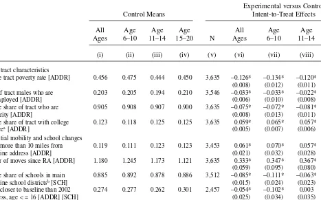
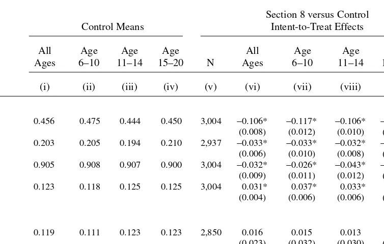
45.6 percent). For those who used the restricted vouchers, this translates to a reduc-tion in neighborhood poverty rate of about 25 percentage points relative to the rate if they had not used the vouchers (the TOT effect). Children in families that moved using an experimental voucher resided an average of 3.1 years (range of 1.3 to 4.6 years for the 25th to 75th percentile) at their new addresses. The differences in poverty rates are largest soon after random assignment and then decline over time.15 Using a separate regression, we estimated the ITT effect of the Section 8 treatment on poverty rates (Table 3, Column 6). The effect was somewhat smaller than the effect for the experimental group, reducing the average poverty rate by 10.6 percent. As the rest of Panel A in Table 2 and in Table 3 show, both treatment offers resulted in chil-dren living in neighborhoods with lower male unemployment, more college-educated adults, and fewer minorities. Effects on neighborhoods were generally stronger for the experimental treatment than for the Section 8 treatment.
Panel B focuses on residential mobility and school switching between randomiza-tion and followup. Children in both the experimental and Secrandomiza-tion 8 groups experi-enced more residential moves than controls, who themselves moved on average at least once. For the experimental group, the voucher offer also led to more moves of at least ten miles from the baseline address.16Treatment group children spent less time than controls attending schools in the five main urban districts associated with the MTO sites, however, there were no statistically significant differences between treat-ment and control groups in terms of the number of schools attended or mid-grade school changes.
The Journal of Human Resources Table 2
Effects on School and Neighborhood Context for the Experimental Group
Experimental versus Control
Control Means Intent-to-Treat Effects
All Age Age Age All Age Age Age
Ages 6–10 11–14 15–20 N Ages 6–10 11–14 15–20
(i) (ii) (iii) (iv) (v) (vi) (vii) (viii) (ix)
A. Census tract characteristics
Average tract poverty rate [ADDR] 0.456 0.475 0.444 0.450 3,635 −0.126* −0.134* −0.120* −0.123* (0.008) (0.012) (0.011) (0.011) Share of tract males who are 0.203 0.205 0.194 0.210 3,546 −0.033* −0.033* −0.022* −0.043*
unemployed [ADDR] (0.006) (0.010) (0.008) (0.009)
Average share of tract who are 0.905 0.908 0.907 0.900 3,635 −0.075* −0.072* −0.081* −0.073*
minority [ADDR] (0.008) (0.013) (0.011) (0.013)
Average share of tract with college 0.123 0.118 0.125 0.125 3,635 0.059* 0.065* 0.057* 0.056*
degreea[ADDR] (0.005) (0.007) (0.006) (0.007)
B. Residential mobility and school changes
Moved more than 10 miles from 0.119 0.111 0.123 0.123 3,453 0.061* 0.070* 0.057* 0.057*
baseline address [ADDR] (0.021) (0.032) (0.028) (0.028)
Number of moves since RA [ADDR] 1.180 1.245 1.173 1.121 3,635 0.333* 0.347* 0.367* 0.285* (0.059) (0.095) (0.080) (0.076) Average share of schools in main 0.885 0.892 0.878 0.886 3,512 −0.085* −0.111* −0.063* −0.081* baseline school districtsb[SCH] (0.015) (0.024) (0.023) (0.022) School closer to baseline than 2002 0.274 0.277 0.262 0.301 2,457 −0.054* −0.102* 0.003 −0.088 address, age <= 16 [ADDR] [SCH] (0.025) (0.034) (0.035) (0.053) Number of schools attended since 2.113 1.447 2.412 2.946 2,944 0.070 0.062 0.087 0.041
Sanbonmatsu, Kling, Duncan, and Brooks-Gunn
665
C. School peers, pupil-teacher ratio and climate
Average share of students eligible for 0.739 0.807 0.754 0.655 2,479 −0.064* −0.082* −0.060* −0.051*
free lunch [SCH], excluding IL (0.009) (0.014) (0.013) (0.014)
Average share of minority 0.912 0.929 0.904 0.903 3,489 −0.046* −0.055* −0.036* −0.048*
students [SCH] (0.007) (0.011) (0.012) (0.012)
Average percentile rank of schools 0.148 0.134 0.151 0.172 2,742 0.044* 0.052* 0.040* 0.035* on state exams [SCH], excluding (0.007) (0.010) (0.009) (0.014) age > 13 for MD, NY
Pupil-teacher ratio [SCH], 18.48 18.41 18.53 18.51 2,681 −0.06 −0.40 −0.17 0.40
excluding MA (0.18) (0.33) (0.30) (0.26)
School climate index, higher 0.646 0.685 0.649 0.610 2,871 −0.010 −0.042* −0.015 0.026
is bettere[SR] (0.011) (0.020) (0.015) (0.022)
Gangs in school or 0.545 0.446 0.592 0.550 3,061 −0.060* −0.054 −0.116* −0.005
neighborhood [SR] (0.022) (0.047) (0.033) (0.034)
Sources: Data sources are indicated in square brackets. ADDR = address history from tracking file linked to Census tract data. Average tract characteristics are the mean for a child’s residences from randomization through 2001, weighted by duration at each address. Values for noncensus years were interpolated or extrapolated from 1990 and 2000 Census data. Share of males unemployed is for the child’s address in 2002 based on 2000 Census data. SCH = school history data linked by school name to school demographics from the National Center for Education Statistics (NCES) and to average scores on state exams from the National School-Level State Assessment Score Database. SR = child self-report, available only for children at least eight years old as of May 31, 2001.
Note: Intent-to-treat (ITT) estimates for “all ages” from Equation 1 and for age groups from Equation 2, using covariates as described in Table 1 and weights described in Section V. Standard errors, adjusted for heteroskedasticity, are in parentheses.
*Statistically significant at the 5 percent level. a. At least an associates or bachelors degree.
b. The five main baseline school districts are Baltimore City, Boston, Chicago, Los Angeles Unified, and New York City. c. Number of schools (grades one through 12) attended since RA.
d. Any mid-grade school change was defined as attending more than one school for the same (unrepeated) grade.
The Journal of Human Resources
Table 3
Effects on School and Neighborhood Context for the Section 8 Group
Section 8 versus Control
Control Means Intent-to-Treat Effects
All Age Age Age All Age Age Age
Ages 6–10 11–14 15–20 N Ages 6–10 11–14 15–20
(i) (ii) (iii) (iv) (v) (vi) (vii) (viii) (ix)
A. Census tract characteristics
Average tract poverty rate [ADDR] 0.456 0.475 0.444 0.450 3,004 −0.106* −0.117* −0.106* −0.095* (0.008) (0.012) (0.010) (0.010) Share of tract males who are 0.203 0.205 0.194 0.210 2,937 −0.033* −0.033* −0.032* −0.032*
unemployed [ADDR] (0.006) (0.010) (0.008) (0.010)
Average share of tract who are 0.905 0.908 0.907 0.900 3,004 −0.032* −0.026* −0.043* −0.027*
minority [ADDR] (0.009) (0.011) (0.012) (0.013)
Average share of tract with 0.123 0.118 0.125 0.125 3,004 0.031* 0.037* 0.033* 0.022*
college degreea[ADDR] (0.004) (0.006) (0.006) (0.006)
B. Residential mobility and school changes
Moved more than 10 miles from 0.119 0.111 0.123 0.123 2,850 0.016 0.015 0.013 0.019
baseline address [ADDR] (0.023) (0.032) (0.030) (0.031)
Sanbonmatsu, Kling, Duncan, and Brooks-Gunn
667
School closer to baseline than 2002 0.274 0.277 0.262 0.301 2,039 −0.049 −0.101* −0.023 0.012 address, age < = 16 [ADDR] [SCH] (0.026) (0.035) (0.037) (0.061) Number of schools attended since 2.113 1.447 2.412 2.946 2,432 0.084 0.081 0.103 0.040
RAc, age < = 16 [SCH] (0.045) (0.053) (0.072) (0.120)
Mid-grade school change since 0.171 0.116 0.193 0.247 2,432 0.019 0.035 0.006 0.015
RAd, age < = 16 [SCH] (0.020) (0.029) (0.029) (0.054)
C. School peers, pupil-teacher ratio and climate
Average share of students eligible for 0.739 0.807 0.754 0.655 2,201 −0.035* −0.062* −0.022 −0.022
free lunch [SCH], excluding IL (0.009) (0.015) (0.015) (0.015)
Average share of minority 0.912 0.929 0.904 0.903 2,840 −0.029* −0.016 −0.025 −0.046*
students [SCH] (0.009) (0.010) (0.013) (0.017)
Average percentile rank of schools
on state exams [SCH], excluding 0.148 0.134 0.151 0.172 2,219 0.020* 0.019* 0.030* 0.003
age > 13 for MD, NY (0.007) (0.009) (0.011) (0.013)
Pupil-teacher ratio [SCH], 18.48 18.41 18.53 18.51 2,149 −0.19 −0.04 −0.22 −0.28
excluding MA (0.21) (0.36) (0.34) (0.30)
School climate index, higher 0.646 0.685 0.649 0.610 2,367 0.009 −0.014 0.017 0.017
is bettere[SR] (0.012) (0.021) (0.017) (0.024)
Gangs in school or 0.545 0.446 0.592 0.550 2,523 −0.019 −0.011 −0.060 0.020
neighborhood [SR] (0.025) (0.052) (0.037) (0.038)
group than for the Section 8 group. Although the administrative data on schools indi-cates differences in school peers between the treatment and control groups, the chil-dren’s perceptions of their schools’ climates generally do not differ between the treatment and control groups.
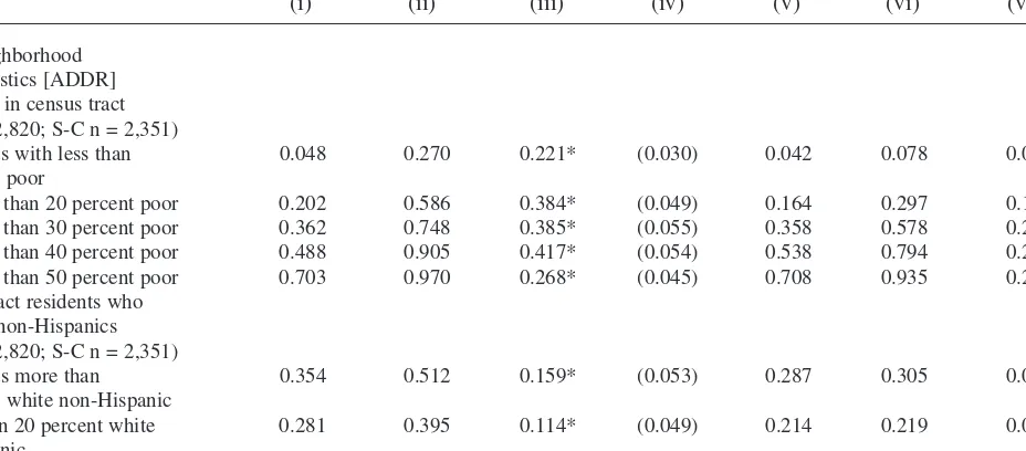
To provide a better sense of what the average changes shown in Tables 2 and 3 rep-resent in terms of the types of neighborhoods and schools of treatment compliers at followup, Table 4 shows the share of treatment compliers in neighborhoods and schools above or below different threshold characteristics. For comparison purposes, the table also shows estimates of the control complier means. Control compliers are those children in the control group whose families would have complied with the treatment if offered it; the neighborhoods and schools of the control compliers repre-sent the counterfactual of what the treatment compliers would have experienced in the absence of the treatment. Although we cannot directly identify the control compliers, we can estimate the characteristics of control compliers under the assumption that the distribution for noncompliers in the treatment and control groups is the same. The shares for the treatment compliers are observed, and the difference in the shares for treatment and control compliers is the TOT effect.
The first row of Table 4 shows that while less than 5 percent of control compliers are estimated to be living in tracts with a poverty rate of less than 10 percent, more than 25 percent of experimental treatment compliers were living in these types of tracts. While roughly half of the control compliers were still living in high poverty neighborhoods (poverty rates of at least 40 percent), this was true for only 10 percent of experimental treatment compliers (see fourth row). The distributions indicate that although the experimental treatment increased the likelihood of a child living in a neighborhood or attending a school that was above the 50thpercentile in rank or had a majority of white non-Hispanics, the treatment induced only a small share of treat-ment complier children who would otherwise not have lived in these types of neigh-borhoods or attended these types of schools to do so: 15 percent of experimental group complier children for tracts above the 50th percentile rank and 8 percent of children for schools above the 50thpercentile.
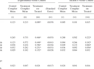
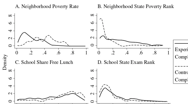
Figure 1 uses kernel density estimates to display the distribution of selected 2002 neighborhood and school characteristics for experimental compliers in comparison to control compliers.18As illustrated by the graph in Panel A of Figure 1, the
Experimental versus Control Section 8 versus Control
Control Treatment Treatment- Control Treatment
Treatment-Complier Treatment-Complier on- (Standard Complier Complier on- (Standard
Mean Mean Treated Error) Mean Mean Treated Error)
(i) (ii) (iii) (iv) (v) (vi) (vii) (viii)
A. Current Neighborhood Characteristics [ADDR] Percent poor in census tract
(E-C n = 2,820; S-C n = 2,351)
share in tracts with less than 0.048 0.270 0.221* (0.030) 0.042 0.078 0.036 (0.020) 10 percent poor
. . . with less than 20 percent poor 0.202 0.586 0.384* (0.049) 0.164 0.297 0.133* (0.042) . . . with less than 30 percent poor 0.362 0.748 0.385* (0.055) 0.358 0.578 0.219* (0.046) . . . with less than 40 percent poor 0.488 0.905 0.417* (0.054) 0.538 0.794 0.256* (0.045) . . . with less than 50 percent poor 0.703 0.970 0.268* (0.045) 0.708 0.935 0.227* (0.036) Percent of tract residents who
are white non-Hispanics (E-C n = 2,820; S-C n = 2,351)
share in tracts more than 0.354 0.512 0.159* (0.053) 0.287 0.305 0.019 (0.043) 10 percent white non-Hispanic
. . . more than 20 percent white 0.281 0.395 0.114* (0.049) 0.214 0.219 0.005 (0.039) non-Hispanic
. . . more than 30 percent white 0.182 0.334 0.152* (0.046) 0.148 0.192 0.044 (0.036) non-Hispanic
Experimental versus Control Section 8 versus Control
Control Treatment Treatment- Control Treatment
Treatment-Complier Treatment-Complier on- (Standard Complier Complier on- (Standard
Mean Mean Treated Error) Mean Mean Treated Error)
(i) (ii) (iii) (iv) (v) (vi) (vii) (viii)
. . . more than 50 percent white 0.123 0.213 0.089* (0.039) 0.085 0.101 0.015 (0.031) non-Hispanic
Statewide neighborhood poverty rank (higher rank indicates less poverty; E-C n = 2,781; S-C n = 2,323)
share in tracts ranking above the 0.265 0.733 0.468* (0.053) 0.280 0.502 0.222* (0.046) 10thpercentile
. . . ranking above the 20thpercentile 0.123 0.572 0.448* (0.041) 0.084 0.266 0.182* (0.038)
. . . ranking above the 30thpercentile 0.038 0.434 0.396* (0.036) 0.049 0.133 0.084* (0.027)
. . . ranking above the 40thpercentile 0.032 0.282 0.251* (0.031) 0.036 0.092 0.056* (0.023)
. . . ranking above the 50thpercentile 0.029 0.182 0.152* (0.028) 0.032 0.064 0.032 (0.019)
B. Current or most recent school characteristics [SCH] Percent of students who are free
lunch eligible, excluding Chicago (E-C n = 1,999; S-C n = 1,783)
share in schools with less than 0.023 0.047 0.024 (0.017) 0.024 0.041 0.016 (0.015) 10 percent eligible for free lunch
Percent of students who are white Non-Hispanic (E-C n = 2,824; S-C n = 2,303)
share in schools more than 0.281 0.411 0.130* (0.044) 0.241 0.285 0.044 (0.037) 10 percent white non-Hispanic
. . . more than 20 percent white 0.171 0.310 0.139* (0.041) 0.158 0.208 0.051 (0.033) non-Hispanic
. . . more than 30 percent white 0.129 0.252 0.122* (0.038) 0.108 0.168 0.061 (0.032) non-Hispanic
. . . more than 40 percent white 0.100 0.192 0.092* (0.033) 0.087 0.116 0.030 (0.028) non-Hispanic
. . . more than 50 percent white 0.073 0.155 0.082* (0.031) 0.055 0.087 0.032 (0.026) non-Hispanic
School rank on statewide exams, excluding age > 13 for MD, NY (E-C n = 2,406; S-C n = 1,970)
share in schools ranking above the 0.575 0.741 0.166* (0.053) 0.538 0.607 0.068 (0.043) 10thpercentile
. . . ranking above the 20thpercentile 0.215 0.439 0.224* (0.047) 0.192 0.275 0.083* (0.035)
. . . ranking above the 30thpercentile 0.143 0.291 0.147* (0.040) 0.119 0.161 0.042 (0.029)
. . . ranking above the 40thpercentile 0.087 0.201 0.114* (0.034) 0.082 0.103 0.022 (0.024)
. . . ranking above the 50thpercentile 0.061 0.137 0.076* (0.029) 0.067 0.076 0.009 (0.020)
Sources: Data sources are indicated in square brackets. ADDR = address history from tracking file linked to 2000 Census tract data. For sample consistency, neighborhood charac-teristics are restricted to children for whom WJ-R scores were available. SCH = school history data linked by school name to data on student demographics from the National Center for Education Statistics and on state test scores from National Longitudinal School-Level State Assessment Score Database. Free school lunch program information was generally not available for Chicago. California reports the number of children receiving free lunch rather than the number eligible. School exam rankings for Maryland and New York exclude children aged 13 years and older as high school exam scores were generally not available at these sites.
Notes: Sample restricted to children aged six to 16. Distribution cutpoints are overlapping. The control complier mean estimated as equal to the treatment complier mean minus the treatment-on-treated effect. The treatment complier mean is unadjusted. Treatment-on-treated effect estimated using two-stage least squares with assignment to a treatment group serv-ing as an instrumental variable for treatment compliance. Standard errors for the treatment-on-treated effect, adjusted for heteroskedasticity, are in parentheses. E-C n = number of observations included in the Experimental-Control comparison. S-C n = number of observations included in the Section 8-Control comparison.
mental treatment led to a distinct shift in neighborhood poverty levels. Graphs in Panels B and D show the distribution of state percentile ranks of neighborhood poverty (with higher ranks indicating less poverty) and school exam scores (with higher ranks indicating higher scores), respectively. These graphs help to compare the changes MTO induced for neighborhoods versus schools. The experimental treatment led to a substantial shift in the distribution of neighborhoods in terms of poverty rank but a more modest change in the distribution of school ranks.
In summary, the offer of a voucher led families to live in neighborhoods that were substantially less poor, had more educated residents, and had somewhat fewer minor-ity residents. The offer also led children to attend schools that performed somewhat Figure 1
Experimental and Control Complier Densities for Neighborhood and School Characteristics
Sources:Tract characteristics are from the 2000 Census and school characteristics from the NCES’s Common Core of Data, the Private School Survey, and the National Longitudinal School-Level Assessment Score Database.
Note:Sample is restricted to children aged six to 16 for whom WJ-R test score data were available. Kernel densities estimates are based on an Epanechnikov kernel and halfwidth of 0.030. For the experimental group, we directly observe the distributions for the overall group, for treatment compliers, and for treatment noncompliers. For the control group, we do not observe who would have complied with the treatment if offered it. However, under the assumption that control noncompliers have the same distribution of characteristics as the experimental noncompliers, we estimate the control complier distribution by subtracting the experimental noncomplier density from the overall control group density (Imbens and Rubin 1997). Neighborhood is defined as the Census tract in which the child lived in 2002 and school as the school attended in 2002. Information on free lunch program was generally not available for Illinois. For comparability, the Kernel density estimates for neighborhood poverty rate and share free lunch eligible were restricted to children with valid data on both measures. School exam scores were generally not available for older children in Baltimore and New York. For comparability, density estimates of state poverty rank and state exam rank exclude children aged 14 and older for Baltimore and New York and only include children with valid data on both measures. Higher rankings represent neighborhoods with lower poverty and schools with higher test scores.
0
A. Neighborhood Poverty Rate B. Neighborhood State Poverty Rank
C. School Share Free Lunch D. School State Exam Rank
Experimental Complier
Control Complier
better on state exams. However, the treatment did not generally lead families to move to white suburban neighborhoods or lead children to attend top performing schools.
VII. Effects on Educational Outcomes
A. Effects on Educational Outcomes, Overall and by Age Group
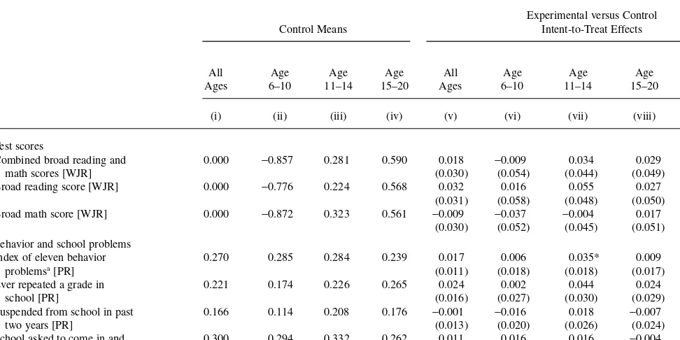
We had hypothesized that moves to lower poverty neighborhoods would lead to improved educational outcomes for children. Panels A of Table 5 and 6 present the estimated effects of the experimental and Section 8 treatments on test scores, our pri-mary outcomes. The first row of each table presents the results for the combined read-ing and math scores. By construction, the mean of the normalized scores for the control group (Column 1) is zero, with a standard deviation of one. To examine scores by age, we divided the sample into three age groups of roughly equal size: aged six to ten, 11 to 14, and 15 to 20. As the control means for the specific age groups in Columns 2 through 4 show, scores rise with age but do so more slowly for the oldest group. The control mean for the youngest children is −0.857, or more than a standard deviation below the mean of 0.281 for the 11 to 14 age group. The coefficient of 0.018 in Column 5 represents the ITT effect of experimental treatment on reading and math for all ages combined, and is less than two hundredths of a standard deviation. The standard error of 0.030 (in parentheses in Column 5) indicates that the ITT estimate is not statistically significant and that we had sufficient statistical power to detect a true effect as small as 0.084 standard deviations (or 2.8 times the standard error of the estimate) 80 percent of the time at the 0.05 level of significance (Bloom 1995).
We had hypothesized stronger effects of the intervention for younger rather than older children. Using a separate regression, we estimate the ITT effects of experi-mental treatment for each age group (see Columns 6 through 8). The treatment effect on the combined reading and math scores is not statistically significant for any of the age groups nor is the coefficient on the linear age interaction (shown in Column 9) statistically significant. The coefficient on the linear age interaction of 0.0016 implies that a ten-year age difference, such as the difference between the effect for 18-year-olds versus eight-year-olds, is associated with only a 0.016 increase (or less than two hun-dredths of a standard deviation) in the magnitude of the ITT effect. Table 6 presents parallel results for the Section 8 treatment and similarly shows no evidence of effects on achievement scores or of an interaction between treatment effects and age.
The Journal of Human Resources Effects on Test Scores and on Behavior and School Problems for the Experimental Group
Experimental versus Control Control Means Intent-to-Treat Effects
Linear
All Age Age Age All Age Age Age Age
Inter-Ages 6–10 11–14 15–20 Ages 6–10 11–14 15–20 action
(i) (ii) (iii) (iv) (v) (vi) (vii) (viii) (ix)
A. Test scores
Combined broad reading and 0.000 −0.857 0.281 0.590 0.018 −0.009 0.034 0.029 0.0016
math scores [WJR] (0.030) (0.054) (0.044) (0.049) (0.0081)
Broad reading score [WJR] 0.000 −0.776 0.224 0.568 0.032 0.016 0.055 0.027 −0.0005 (0.031) (0.058) (0.048) (0.050) (0.0084) Broad math score [WJR] 0.000 −0.872 0.323 0.561 −0.009 −0.037 −0.004 0.017 0.0023
(0.030) (0.052) (0.045) (0.051) (0.0081) B. Behavior and school problems
Index of eleven behavior 0.270 0.285 0.284 0.239 0.017 0.006 0.035* 0.009 0.0005
problemsa[PR] (0.011) (0.018) (0.018) (0.017) (0.0024)
Ever repeated a grade in 0.221 0.174 0.226 0.265 0.024 0.002 0.044 0.024 0.0026
school [PR] (0.016) (0.027) (0.030) (0.029) (0.0039)
Suspended from school in past 0.166 0.114 0.208 0.176 −0.001 −0.016 0.018 −0.007 0.0003
two years [PR] (0.013) (0.020) (0.026) (0.024) (0.0032)
School asked to come in and 0.300 0.294 0.332 0.262 0.011 0.016 0.016 −0.004 0.0004 talk about problemsb[PR] (0.018) (0.032) (0.031) (0.034) (0.0052)
Sources: Data sources are indicated in square brackets. WJR = Woodcock Johnson-Revised battery of tests. PR = parental report.
Note: Intent-to-treat (ITT) estimates for all ages from Equation 1 and estimates for age groups from Equation 2, using covariates as described in Table 1 and weights described in Section V. Linear age interaction is the estimated additional treatment effect from Equation 3 of an additional year of age. Standard errors, adjusted for heteroskedasticity, are in parentheses.
* Statistically significant at the 5 percent level.
a. The behavior problem index is the fraction of the following eleven items that the adult respondent reported were “often” or “sometimes” true for the child: “cheats or tells lies,” “bullies or is cruel or mean to others,” “hangs around with kids who get into trouble,” “is disobedient at school,” “has trouble getting along with teachers,” “has difficulty concentrating, cannot pay attention for long,” “is restless or overly active, cannot sit still,” “has a very strong temper and loses it easily,” “disobedient at home,” “has trouble getting along with other children,” and “withdrawn, does not get involved with others.”
Sanbonmatsu, Kling, Duncan, and Brooks-Gunn
675
Section 8 versus Control
Control Means Intent-to-Treat Effects
Linear
All Age Age Age All Age Age Age Age
Inter-Ages 6–10 11–14 15–20 Ages 6–10 11–14 15–20 action
(i) (ii) (iii) (iv) (v) (vi) (vii) (viii) (ix)
A. Test scores
Combined broad reading and 0.000 −0.857 0.281 0.590 0.000 −0.046 −0.031 0.073 0.0064
math scores [WJR] (0.032) (0.055) (0.047) (0.056) (0.0081)
Broad reading score [WJR] 0.000 −0.776 0.224 0.568 0.031 0.009 0.008 0.072 0.0011 (0.034) (0.062) (0.051) (0.058) (0.0088) Broad math score [WJR] 0.000 −0.872 0.323 0.561 −0.037 −0.083 −0.074 0.046 0.0069
(0.032) (0.055) (0.047) (0.056) (0.0080) B. Behavior and school problems
Index of eleven behavior 0.270 0.285 0.284 0.239 0.006 0.005 0.011 0.001 −0.0007
problemsa[PR] (0.012) (0.018) (0.019) (0.019) (0.0025)
Ever repeated a grade 0.221 0.174 0.226 0.265 −0.020 −0.010 −0.007 −0.042 −0.0035
in school [PR] (0.017) (0.030) (0.032) (0.030) (0.0040)
Suspended from school in past 0.166 0.114 0.208 0.176 −0.010 −0.009 0.012 −0.033 −0.0042
two years [PR] (0.015) (0.021) (0.029) (0.025) (0.0033)
School asked to come in and 0.300 0.294 0.332 0.262 0.008 0.003 0.016 0.005 0.0034
talk about problemsb[PR] (0.021) (0.034) (0.036) (0.038) (0.0057)
The Journal of Human Resources Effects on School Engagement and Special Classes for the Experimental Group
Experimental versus Control
Control Means Intent-to-Treat Effects
Linear
All Age Age Age All Age Age Age Age
Inter-Ages 8–10 11–14 15–18 Ages 8–10 11–14 15–18 action
(i) (ii) (iii) (iv) (v) (vi) (vii) (viii) (ix)
A. School engagement
Always pays attention in 0.548 0.598 0.560 0.487 0.022 0.077 −0.025 0.051 −0.0060
class [SR] (0.023) (0.042) (0.032) (0.041) (0.0077)
Works hard in school [SR] 0.573 0.669 0.584 0.477 −0.000 0.064 −0.015 −0.028 −0.0113 (0.023) (0.041) (0.032) (0.041) (0.0078) Reads at least five hours/week 0.261 0.254 0.250 0.283 −0.004 −0.033 −0.011 0.029 0.0096
excluding schoolwork [SR] (0.021) (0.038) (0.029) (0.037) (0.0071)
Late less than once a month [SR] 0.482 0.592 0.504 0.358 0.013 −0.038 0.040 0.018 0.0055 (0.023) (0.044) (0.032) (0.039) (0.0078) B. Special classes
Class for gifted students or did 0.115 0.120 0.117 0.109 0.019 0.008 0.025 0.018 0.0006
advanced work in past (0.014) (0.027) (0.021) (0.026) (0.0052)
two years [PR]
Special class or help for learning, 0.255 0.250 0.266 0.241 0.019 0.053 0.008 0.006 −0.0034
behavioral or emotional (0.018) (0.041) (0.029) (0.030) (0.0065)
problems in past two years [PR]
Sources: Data sources are indicated in square brackets. SR = child self-report. PR = parental report.
Sanbonmatsu, Kling, Duncan, and Brooks-Gunn
677
Experimental versus Control
Control Means Intent-to-Treat Effects
Linear
All Age Age Age All Age Age Age Age
Inter-Ages 8–10 11–14 15–18 Ages 8–10 11–14 15–18 action
(i) (ii) (iii) (iv) (v) (vi) (vii) (viii) (ix)
A. School engagement
Always pays attention 0.548 0.598 0.560 0.487 0.026 0.031 −0.007 0.074 0.0000
in class [SR] (0.025) (0.045) (0.037) (0.045) (0.0085)
Works hard in school [SR] 0.573 0.669 0.584 0.477 0.001 0.041 −0.024 0.008 −0.0103 (0.024) (0.044) (0.036) (0.044) (0.0085) Reads at least five hours/week 0.261 0.254 0.250 0.283 0.000 −0.035 0.003 0.023 0.0073
excluding schoolwork [SR] (0.023) (0.042) (0.032) (0.043) (0.0081) Late less than once a 0.482 0.592 0.504 0.358 0.017 0.004 0.064 −0.041 −0.0072
month [SR] (0.026) (0.050) (0.037) (0.043) (0.0085)
B. Special classes
Class for gifted students or did 0.115 0.120 0.117 0.109 0.002 0.004 0.007 −0.006 −0.0013
advanced work in past (0.015) (0.030) (0.021) (0.026) (0.0050)
two years [PR]
Special class or help for 0.255 0.250 0.266 0.241 0.013 0.043 0.022 −0.024 −0.0067 learning, behavioral or (0.020) (0.041) (0.032) (0.033) (0.0071) emotional problems in past
two years [PR]