Cycle Consequences
Exploiting a Natural Experiment
V. Joseph Hotz
Susan Williams McElroy
Seth G. Sanders
A B S T R A C T
We exploit a “natural experiment” associated with human reproduction to identify the causal effect of teen childbearing on the socioeconomic attain-ment of teen mothers. We exploit the fact that some women who become pregnant experience a miscarriage and do not have a live birth. Using mis-carriages an instrumental variable, we estimate the effect of teen mothers not delaying their childbearing on their subsequent attainment. We find that many of the negative consequences of teenage childbearing are much smaller than those found in previous studies. For most outcomes, the adverse consequences of early childbearing are short-lived. Finally, for annual hours of work and earnings, we find that a teen mother would have lower levels of each at older ages if they had delayed their childbearing.
I. Introduction
Over the past several decades, social scientists have documented a strong statistical association between the age at which a woman has her first child and economic and social indicators of her subsequent well-being. Most of these studies
V. Joseph Hotz is a professor of economics at the University of California, Los Angeles. Susan Williams McElroy is an associate professor of economics and education policy at the University of Texas at Dallas. Seth G. Sanders is a professor of economics at the University of Maryland. This research was supported, in part, by NICHD Grant No. R01 HD-31590. The authors wish to thank Sarah Gordon, Stuart Hagen, Terra McKinnish, Charles Mullin, Carl Schneider, and Daniel Waldram for able and conscientious research assistance on this project. They wish to thank Robert Moffitt, Frank Furstenberg, Arleen Leibowitz, John Strauss, Susan Newcomer, Arline Geronimus and participants of the Institute for Research on Poverty Workshop on Low Income Populations for helpful comments on an earlier draft. They also thank Frances Margolin, Hoda Makar, Simon Hotz, Leonard Stewart, Jr., and Kruti Dholakia for editorial assistance. The authors are grateful to Saul Hoffman for bringing to our attention a set of systematic errors in the deflating of the monetary variables used in our analyses to real terms in a previous draft. All of these errors have been corrected. The authors especially wish to thank Robert Willis for numerous helpful discussions during the course of this study. All remaining errors are the responsibility of the authors.
[Submitted October 2002; accepted July 2004]
find that women who bear children as teenagers are subsequently less likely to com-plete high school, less likely to participate in the labor force, more likely to have low earnings, and less likely to marry than are women who do not have children as teenagers. Furthermore, adolescent mothers, and their children, are likely to spend a substantial fraction of their lifetimes in poverty and are more likely to rely on gov-ernment support. (See Upchurch and McCarthy 1990 and Card 1981).
The important question is whether these statistical associations reflect a causal effect of early childbearing on the subsequent economic and demographic outcomes of teen mothers. It is possible that these associations simply reflect differences between the type of women who bear children as teens and those who avoid it. For example, teenage mothers typically were raised in families that were especially disadvantaged based on a number of measurable indicators. Because teenage mothers tend to be from families of lower socioeconomic status, and socioeconomic status of parents and children appear to be themselves correlated, it is difficult to assess whether a teen birth is respon-sible for the poorer outcomes of teenage mothers or whether a teen mother’s subsequent outcomes are attributable to the socioeconomic conditions in which she was reared.
The key issue in attempts to estimate the causal effect is how to estimate reliably the counterfactual state to the observed outcomes of teen mothers: namely, what would have been the adolescent mother’s outcomes if she had not had a child as a teen? Varieties of econometric strategies have been used to estimate this counter-factual outcome. The most common approach is to control for observable factors, typ-ically using regression methods, that account for the lower economic status of teenage mothers when they were growing up and to attribute any differences in outcomes between teenage mothers and other women, net of these observables, to the causal effects of teenage childbearing. (See Waite and Moore 1978, Card and Wise 1978, Hofferth and Moore 1979, Upchurch and McCarthy 1990, Marini 1984, and McElroy 1996a, 1996b as examples of this strategy.) The validity of this approach requires that, conditional on these observable factors or covariates, a woman’s status (teen mother or not a teen mother) be uncorrelated with all remaining and unobservable factors that might influence the outcomes under consideration. Clearly, this condition is strong and, as we show below, its validity is dubious for a variety of reasons.
A second econometric methodology uses the outcomes of an adolescent mother’s sisters who did not have a child as a teenage to construct counterfactual outcomes for teen mothers. (See Geronimus and Korenman 1992, 1993 and Hoffman, Foster, and Furstenberg 1993). Comparing the outcomes of a teenage mother to her sister who did not have a child as a teen has the intuitive appeal of controlling for a variety of pre-teen characteristics and factors, both observed and unobserved, that were com-mon to the environments—family, socioeconomic, and otherwise—in which these two women were reared. The challenge to the validity of this sibling-differences or sister-differences approach is that the socioeconomic conditions facing sisters and the parental inputs received by sisters may differ if family circumstances change over time and with the childrearing experiences of their parents.1
A third econometric approach attempts to model explicitly the joint process deter-mining the woman’s decision to bear a child as a teenager as well as the maternal out-come of interest, such as, education, labor supply, or poverty status. (See Ribar 1992, 1994, and Lundberg and Plotnick 1989 as examples of this strategy.) Such studies typ-ically rely on rational choice models that hypothesize that women with lower returns to work and education are the ones that have children as teens. Such models maintain an equally strong, albeit different, set of assumptions in order to identify the effects of early childbearing: namely, that the model of these behavioral decision processes adequately characterizes both the teenage childbearing and outcomes decisions and how they interact.
Finally, the work of Grogger and Bronars (1993) provides a fourth approach that makes use of a “naturally occurring” experiment to estimate causal effects of early childbearing.2In particular, Grogger and Bronars make use of the fact that some teenage
mothers have twins at their first birth rather than a single child. Because the occurrence of twins from a typical conception can be viewed, by and large, as random, it as if the “extra” child was randomly assigned. These authors compare the outcomes of teen mothers whose first birth is twins with those whose first birth is a single child to esti-mate a causal effect of this extra child. While an innovative approach, the Grogger-Bronars “twins” method estimates a causal effect that is different from the one that is the subject of much of the literature and, as will be made clear below, is also different from the one considered in this article. Most of the previous literature on the (causal) effects of teenage childbearing seeks to estimate the effect of having at least one child as a teenager relative to having no children as a teenager. In contrast, the Grogger and Bronars study identifies the marginal effect of having two children as a teen compared to having one child. Grogger and Bronars recognize this potentially important difference in their work. They argue that if having one more child lowers the outcomes of teen mothers, the effect of having only one child as a teen is likely to be at least as large.
In this article, we exploit an alternative “natural experiment” associated with human reproduction to measure counterfactual outcomes: namely, what would have happened to a teen mother if she had not had her first birth as a teen? In particular, we exploit the fact that some women who become pregnant as teenagers experience a miscarriage (spontaneous abortion) and thus do not have a birth.3The physiology of human
repro-duction implies that some miscarriages occur at random resulting from the formation of abnormal fetal chromosomes at the time of conception, which causes fetal expulsion early in a pregnancy.4Because miscarriages are close to random, we argue for using
miscarriages as an instrument in order to obtain unbiased estimates of the causal effects of teenage childbearing on indicators of women’s subsequent socioeconomic attain-ment and maternal outcomes.
In the next section, we describe the data from the National Longitudinal Survey of Youth, 1979 (NLSY79) that we use in this study. In Section III, we lay out our use of miscarriages as a natural experiment and show how miscarriages can be used to form
2. Bronars and Grogger (1995) use this same twins strategy to identify the causal effect of women having an extra out-of-wedlock birth on the socioeconomic attainment of such mothers.
3. Using a testing strategy for assessing the validity of instruments, developed in Hotz, Mullin and Sanders 1997, we show that one cannot reject the validity of miscarriages as an instrument.
an instrumental variables (IV) estimator for the effect of teen births on maternal out-comes. Therein, we also consider the threats to our inferences due to the possibility that some miscarriages are not random, and that fertility events, especially miscarriages and induced abortions, are likely to be underreported in survey data. We discuss how we address these complications and report relevant findings from our previous work. In Section IV, we present our basic findings of the effect of teenage childbearing on a wide variety of subsequent economic and demographic outcomes, including educational attainment, subsequent fertility and marriage rates, labor market success, personal and spousal income, the incidence of living in poverty, the likelihood of receiving various forms of public assistance, and the dollar amounts of the benefits from these programs. Our major finding is that many of the apparent negative consequences of teenage childbearing on the subsequent socioeconomic attainment of teen mothers are much smaller than those found in studies that use alternative methodologies to identify the causal effects of teenage childbearing. We also find evidence that teenage mothers earn more in the labor market at older ages than they would have earned if they had delayed their births. Comparing our IV estimates with estimates based on ordinary least squares (OLS) regression methods that control for observable characteristics, we find that the apparent negative consequences previously attributed to teenage child-bearing appear to be the result of the failure to account for other, unobservable fac-tors. In Section V, we offer some concluding comments on our analysis.
II. Data and Samples Used
In this study, we use data from the National Longitudinal Survey of Youth (NLSY79) to estimate the causal effects of teenage childbearing in the United States. The NLSY79 is a nationally representative sample of young men and women who were between the ages of 14 and 21 years old as of January 1, 1979. Thus, the women in our study were teenagers (ages 13 to17) during the years 1971 and 1982.
Respondents have been interviewed annually in the years 1979 through 1992, the last year used in our analysis. The female respondents were asked a range of questions about all of their pregnancies and births, as well as about their marital arrangements, educational attainment, labor force experiences, family income, and participation in various welfare programs.
The NLSY79 contains a cross-sectional sample designed to be representative of women in the non-institutionalized civilian population in the United States for the above-noted birth cohorts, as well as supplemental samples of blacks, Hispanics, disad-vantaged whites, and women who were enlisted in the military in 1979. As is common in many analyses using the NLSY79, we eliminate the economically disadvantaged white supplementary and military samples from our analysis.5We refer to this sample,
those in the random sample and the black and Hispanic supplemental samples, as the
All Womensample. This sample contains 4,926 women, of which 3,108 were from the random sample, and 1,067 and 751 women, were in the black and Hispanic supple-mental samples, respectively.
In Table 1, we provide summary statistics on background characteristics—most of which are measured when these women were age 146—for the All Women sample.
These statistics are calculated using weighted data—as are all of the estimates pre-sented in the remainder of this article—where we use base-year (1979) weights to account for the original design of the sample drawn in this study and the differential probabilities of completing the base-year interviews.7We divide the sample into teen
mothers and women who did not have births as a teenager. Teen mothers came from much more disadvantaged backgrounds than did women who did not have births as teens. For example, teenage mothers grew up in homes that were poorer. The average annual income of the households in which teenage mothers lived in 1978 was $30,532 versus $50,717 (in 1994 dollars) for their non-teen mother counterparts. Teen moth-ers had parents who were less educated. The fathmoth-ers of women who later became teenage mothers completed an average of 9.9 years of schooling versus 11.9 years of schooling for the fathers of other women. Teen mothers were more likely to grow up in single-parent families (31 percent versus 16 percent). In addition, they were more likely to have been in a family living on welfare when growing up (19 percent versus 11 percent) than women who did not have a child as a teen. Clearly, teenage mothers were markedly different from women who delayed childbearing into adulthood in many ways we can observe.
We next consider the subsample of women who experienced at least one preg-nancy while they were teens, that is, prior to their eighteenth birthday. We refer to this subsample as the Teen Pregnancysample. The Teen Pregnancy sample consists of 1,042 women, of whom 74.7 percent (778) had a pregnancy that ended in a birth8
and 25.3 percent (264) had a pregnancy that did not end in a birth. Women whose pregnancies did not end in a birth can be further divided into the 192 (18.4 percent) who had an induced abortion and the 72 (6.9 percent) whose pregnancies ended in a
6. The two exceptions to this in Table 1 are the annual income of the household in which a woman resided, which was taken in 1978, and the woman’s score on the Armed Forces Qualifying Test (AFQT), which was administered to all women in the NLSY79 in 1981.
7. We wish to thank Jay Zagorsky of the Center for Human Resource Research at the Ohio State University for providing us with the appropriate base-year weights for our particular combination of the cross-sectional and supplemental samples. (The appropriate set of weights for this combination of subsamples are not avail-able in the public-release versions of the NLSY79.) We note that the NLSY79 also provides yearly updated weights to take account of nonresponse at each interview using a set of post-stratification adjustment proce-dures described in Frankel, McWilliams and Spencer (1983). In an extensive evaluation of the NLSY79 data, MaCurdy, Mroz and Gritz (1998) find differences in estimating the distributions of labor market earnings and hours of work when using weighted versus unweighted data. However, they also find that it does not matter whether one weights the data with the 1979 base weights or year-by-year versions of these weights that adjust for attrition over the course of the study.
miscarriage.9Table 2 presents statistics on the same background characteristics dis-played in Table 1 for the Teen Pregnancy sample by how their first pregnancy was resolved. Note that while the subsample of women whose first pregnancy before age 18 did notend in a birth had background characteristics that were more similar to those of teen mothers than to characteristics of women who were not teen mothers (see Table 1). As shown in Table 1 and Column 3 of Table 2, these two subgroups (teen mothers and women with first pregnancies prior to age 18 that did not end in a birth) have quite different characteristics. As revealed in Columns 3 and 4 in Table 2, (women whose first pregnancies ended in an abortion and miscarriage, respec-tively), this dissimilarity in background characteristics is due primarily to the women whose first pregnancies were resolved with an abortion. In particular, the abortion group has characteristics that are much more similar to those of women who did not have teen births (see Table 1) than they are to those of teen mothers.10
9. The details of how we constructed the pregnancy and pregnancy resolution variables from the informa-tion available in the NLSY79 data are available in a detailed Data Appendix that can be found at www.econ. ucla.edu/~hotz/teen_data.pdf.
10. Cooksey (1990) also documents that teens who abort their pregnancies tend to come from higher socio-economic backgrounds and/or have higher sociosocio-economic attainment (for example, more educated) than are teenage women who carry their pregnancies to term.
Table 1
Background Characteristics of Teenage Mothers and Women Who Delayed Childbearing until after Age 18
Teenage Mothers Not Teenage Mothers
Standard Standard
Characteristic Mean Duration Mean Duration
Black 0.33 0.47 0.12 0.33
White 0.58 0.49 0.82 0.39
Hispanic 0.09 0.29 0.06 0.24
Family on welfare in 1978a 0.19 0.39 0.11 0.31
Family income in 1978b $30,532 $22,401 $50,717 $31,841
In female-head household 0.20 0.40 0.12 0.33
at age 14
In intact household at age 14 0.69 0.46 0.84 0.37
Mother’s education 9.88 2.86 11.67 2.76
Father’s education 9.94 3.37 11.91 3.56
AFQT scorea 25.81 21.39 49.58 27.49
Number of observations 603 4,323
Data Source: NLSY79, All Women sample; weighted estimates. a. Estimates are expressed in 1994 dollars.
Hotz, McElro
y, and Sanders
689
All Women First Pregnancy First Pregnancy First Pregnancy First Pregnancy P-Value, Pregnant before 18 before 18 did not before 18 ended before 18 ended
Differ-before 18 ended in Birth end in Birth in Abortion in Miscarriage ence in
(1) (2) (3) (4) (5) Meansa
Standard Standard Standard Standard Standard Mean Deviation Mean Deviation Mean Deviation Mean Deviation Mean Deviation
Black 0.27 0.44 0.30 0.46 0.18 0.38 0.16 0.36 0.26 0.44 0.838
White 0.65 0.48 0.61 0.49 0.76 0.43 0.79 0.41 0.63 0.49 0.773
Hispanic 0.08 0.28 0.09 0.29 0.07 0.25 0.05 0.22 0.11 0.32 0.353
Family on welfare 0.16 0.37 0.19 0.39 0.09 0.29 0.09 0.28 0.11 0.32 0.127
in 1978b
Family income $37,551 $28,201 $32,267 $23,217 $47,975 $33,809 $52,774 $34,999 $27,441 $16,919 0.003 in 1978b
In female-headed 0.18 0.39 0.19 0.39 0.16 0.36 0.14 0.34 0.23 0.42 0.361
family at age 14
In intact household 0.72 0.45 0.71 0.45 0.75 0.43 0.78 0.42 0.64 0.48 0.189
at age 14
Mother’s education 10.41 2.74 10.00 2.84 11.36 2.23 11.70 2.15 10.15 2.07 0.401
Father’s education 10.47 3.33 9.93 3.33 11.67 3.02 11.89 2.93 10.70 3.23 0.620
AFQT score 31.55 23.65 27.30 21.92 41.63 24.59 44.38 24.52 31.59 22.30 0.990
Number of 1,042 778 264 192 72
observations
Percent of those 74.7% 25.3% 18.4% 6.9%
pregnant before age 18
In contrast, the women whose (first) teen pregnancies were resolved via a mis-carriage are much more similar to teen mothers than they are to any of the other potential comparison groups displayed in Tables 1 and 2. This similarity in observ-able characteristics for the two groups is indicative of why the estimates of causal effects of teenage childbearing derived from our natural experiment presented below differ from estimates found in the previous literature. In the next section, we provide a more formal justification for the appropriateness of using the data on women who experience miscarriages as teens when estimating the counterfactual outcomes for teen mothers to identify the causal effect of teenage childbearing on maternal outcomes.
III. The Use of Miscarriages as a Natural Experiment
(and as an Instrumental Variable)
Consider the population of women who first become pregnant as ado-lescents and, thus, are at risk to become a teen mother. A pregnancy can be resolved in one of three ways: the occurrence of a birth, an induced abortion, or a miscarriage. Let Dbe the indicator of how the pregnancy is resolved, where D= B(birth), A (abor-tion), or M(miscarriage). For now, assume that miscarriages are beyond the control of women, while the births and abortions represent choices by those who did not experience a miscarriage.11Among women who experience miscarriages, we define a
woman’s latent typeas the way a woman would chooseto resolve a pregnancy if she did not experience the miscarriage. Let D*= B*if a woman’s latent type is to have a birth and D*= A*if her latent type is to have an abortion. Finally, let Ydenote out-comes women experience as an adult age, that is, at ages greater than 18, and Yk(k=
B, A, or M) denote the outcome conditional on the way in which the pregnancy was resolved, and Yk*(k*= B*or A*) denote the outcome that would occur if a woman had a particular latent pregnancy type.12 The outcomes associated with a woman’s
latent type are hypothetical in that the econometrician can not observe a woman’s latent type.
We define the causal effect of interest in this article as the average effect of a woman having a birth as a teen versus delaying it—either to an adult age or permanently—on adult outcomes for the population of women whose first birth is as a teen. More pre-cisely, we are interested in identifying and estimating
(1) β= E(YB−YB*⎜D=B).
Angrist and Imbens (1991) refer to this type of causal effect as the selected average treatment effect(SATE), where “selected” refers to the fact that the causal effect applies to a selected population.13In our context, the selected population is women
who have their first births as a teenager. Because of this selectivity in the population
11. We note that most miscarriages occur very early in a pregnancy so that they usually occur before women could choose to have an induced abortion.
and because we do not presume that pregnancies are random events, we cannot make inferences about the causal effects of early childbearing for a randomly chosen teenage woman in the United States.14 Nonetheless, identifying the causal effect
defined in Equation 1 is of interest for at least two reasons. First, as we will argue below, βis more readily identified from available data than is the speculative causal effect of the consequences of a teen birth among a randomly selected woman from the population of all women, regardless of teen childbearing status. Second, identi-fying βenables one to assess the potential consequences of completely eliminating teenage childbearing in the United States. Assessing such effects provides a bench-mark against which to judge the potential benefits that could be derived from any particular policy mechanism directed at reducing the incidence of teenage child-bearing.
It is apparent from Equation 1 that the problem of estimating βcenters on the iden-tification of E(YB*⎢D= B), sinceE(YB⎢D= B) is readily obtained from data on women
who had their first births as teenagers. Ideally, one would like to use data on Yfor women who have miscarriages as teens but for which D*= B*. Unfortunately, we cannot identify the members of this group. However, we do observe the outcomes for women who miscarry, denoted by YM, which provides some information about the
women in the YB*group. In particular, E(YM) is equal to
(2) E(YM)= P* E(YB*)+(1 −P*)E(YA*),
where the weighting factor, P*, is the proportion of pregnant women who would have had a birth if they not miscarried. Solving Equation 2 for the average outcome for latent-birth women, E(YB*), we obtain
(3) E(YB*)=
E(YM)−(1−P*)E(YA*)
P*
While E(YM) can be identified (and consistently estimated) from observable data on
women who have a miscarriage as a teen, we cannot identify (or readily estimate) either E(YA*) orP*since doing so would also require knowing each woman’s latent
pregnancy type when she was a teen.
If (i) all miscarriages are random and (ii) all fertility events are correctly reported, then the fraction of women who would have carried the pregnancy to term among women who miscarried (P*) must equal the fraction of women who did carry the pregnancy to term among women who do not miscarry (P). That is, P* = P.15
Furthermore, if (iii) having a miscarriage or an abortion has the same direct effect on
Y, then, on average, the outcomes for women who have abortions will be equal to
14. By analogy to the program evaluation literature, the causal effects we focus on are analogous to making inferences about the effect of a program on those who choose to participate and need not apply to a randomly selected individual being required to participate in program. See Heckman (1992) for a discussion of the dis-tinctions between and usefulness of various treatment effect definitions.
those of women in the latent-abortion group.16That is, E(Y
A*) = E(YA).17Under these
conditions, E(YB*) is equal to:
(4) E (YB*)=
E(YM)−(1−P)E (YA)
P
It follows that bcan be written as a function of statistics that are identified (and, thus, readily estimated) from observable data. In particular,
β*=E (YB−YB* | D=B)
=PE(YB)+(1−P)E(YA)−E(YM)
P
(5)
=E(Y~M−YM)
P
= Cov(Y, ˜M) Cov( ˜B, ˜M)
where E(Y~M) is the average outcome for women who did not miscarry—since E(Y~M)
≡PE(YB) +(1−P)E(YA)—and ˜Band M˜ denote indicator variables equal to 1 if a women
D= Band M, respectively, and 0 otherwise.18
Given the definition in Equation 5, it follows that a simple Instrumental Variables (IV) estimator can be formed for β. Let Y−~Mdenote the sample mean of Yfor those
women (observations in the data set) who do not experience a miscarriage, Y−~Mdenote
the sample mean for those women who do experience miscarriages, and Pˆdenote the sample proportion of women who do not experience a miscarriage. Then it follows that an IV estimator for βis
Y−~M−Y
−
M
(6) bˆIV
1 = Pˆ
= Cov(Y, ˜M)
Cov(B˜, M˜ )
where Cov(w1, w2) denotes the sample covariance between variables w1and w2. It
fol-lows from Equation 6 that the miscarriages variable (M˜) serves as an instrument for teen births (˜B) in estimating the causal effect on outcomes (Y).
As noted above, the validity of the estimator in Equation 6 hinges on maintaining the three conditions noted above (ithrough iii). The validity of each is subject to debate. For example, epidemiological studies have found that smoking and drinking
〈
〈
〈
16. On average, the outcomes for women who have abortions will be equal to those of all women in the latent-abortion group if an latent-abortion and a miscarriage affected Yonly through the absence of a child. Alternatively, a miscarriage and an abortion could have a direct effect on Yas long as the effects were equal.
during pregnancy significantly increase the incidence of miscarriages.19Furthermore,
such behaviors are likely to be correlated with such subsequent outcomes for women as labor market earnings. Thus, some miscarriages may fail the exclusion restrictions required of a proper instrumental variable estimator applied to some or all maternal outcomes. Other challenges to the validity of these conditions are examined in Hotz, Mullin and Sanders (1997), who systematically assess the consequences of violating each of these conditions for the estimation of the causal effect of teenage childbear-ing (b). They show that in the presence of violations to (i)–(iii) one cannot point iden-tify the casual effect in Equation 1—and, thus, ensure the consistency of the IV estimates in Equation 6—without knowledge of a woman’s latent type among women who experience miscarriages.
However, Hotz, Mullin, and Sanders (1997) also demonstrate that one can form non-parametric bounds on β, even when none of these conditions holds. Furthermore, these bounds are tightas defined by Horowitz and Manski (1995) and can be derived and non-parametrically estimated, using auxiliary information on the proportion of miscarriages that are random and on the incidence of underreporting in surveys of abor-tion and miscarriage events. In their empirical investigaabor-tion on a more limited set of outcomes than considered in this article-specifically educational attainment, annual hours of work, and earnings—Hotz, Mullin, and Sanders (1997) find that the esti-mated bounds are sufficiently tight to reject the null hypotheses on the signs of the causal effects. For example, the lower bound on the estimated effect of teenage child-bearing on earnings is found not to be less than zero.
Using their estimated bounds on causal effects, Hotz, Mullin, and Sanders (1997) also are able to provide a direct assessment of the validity of the simple IV estimator in Equation 6. Since the bounds constructed in Hotz, Mullin, and Sanders (1997) col-lapse to the simple IV point estimates when assumptions (i)–(iii) hold, a clear indica-tion that they are violated would be if the IV estimates lie outside of the nonparametric bounds. In 832 tests at 13 different ages at which outcomes were measured for the same sample of women used in this article, the simple IV estimator is rejected only 21 times at the 0.05 level.20
Based on the findings from the above study, we maintain the assumptions neces-sary for miscarriages to be a valid instrument for teenage births on a more complete set of maternal outcomes than considered in that study. A further piece of supporting evidence for using miscarriages as an instrument is provided by a comparison of the background characteristics for the samples of women whose first pregnancy occurred prior to age 18 and those women who reported that their pregnancy ended in a mis-carriage. Recall that summary statistics for a set of background characteristics for each of these two groups are presented in Table 2. If miscarriages are random, there should be no difference, on average, in the characteristics of women who miscarry
19. See Kline, Stein, and Susser (1989) for a review of these findings. We note that epidemiologists have not found evidence of statistical associations between other behaviors, such as a woman’s socioeconomic status, her nutrition, or her drug use, and the incidence of miscarriage, although these factors are found to affect birth weight. The latter findings also are summarized in Kline, Stein and Susser (1989).
and those women who become pregnant as teens. In the last column of Table 2, we present the p-values for tests of differences in the means of the background vari-ables of these two groups. With the exception of the income of the woman’s family in 1978, there are no statistically significant differences in the mean values of prepreg-nancy background characteristics of women who became pregnant before age 18 and did not miscarry and those who became pregnant before age 18 and miscarried. The striking similarity of these two groups of women in terms of their prepregnancy back-ground characteristics provides substantive evidence that women who became preg-nant as teens and miscarried constitute an appropriate control group to women who were pregnant as but did not miscarry.
In the next section, we present two sets of IV estimates of the causal effects of teenage childbearing. The first set estimates the causal effects on maternal outcomes measured at a particular adult age a, based on the following linear regression function,
(7) Yia= αa+ βa˜Bi+ θaXi+ εia,
where Yiadenotes the ith woman outcome as of age a, eiais a disturbance term, aais
the intercept, and βais the age-specific causal effect of teenage childbearing and
Xidenotes a vector of covariates, measured when the woman is a teen. We estimate
three variants of Equation 7. One variant includes no covariates. A second controls for such a set of behavioral factors that the epidemiological literature has documented to be correlated with the incidence of miscarriages. These include, for example, whether the woman reported that she smoked or drank alcohol prior to her first preg-nancy or age 18. A third variant of Equation 7 also includes the personal and family background characteristics displayed in Tables 1 and 2, in an attempt to improve the precision of our estimates of βa. For each of these specifications, we use Mito
instru-ment for Biin order to produce IV estimates of βa. For comparison, we also present
estimates of βausing ordinary least squares (OLS) methods.
As noted in the Introduction, we are particularly interested in how the effect of teenage childbearing varies over a teen mother’s life cycle. To produce these age-specific estimates, we use the following modified version of the regression age- specifica-tion in Equaspecifica-tion 7,
(8) Yia =(α18+ β18˜Bi)I
18
ia+(α19+ β19˜Bi)I
19
ia+...
+ (α35+ β35˜Bi)I
35
ia+ θXi + ia ,
where Iiaa¢is an indicator variable equal to 1 if a= a′and equal to zero otherwise and,
to reduce the number of parameters estimated, we constrain qto not vary with age.21
We use the method of Huber (1967) to correct the estimated standard errors of param-eter estimates for the temporal dependence of age-specific outcomes for the same woman.
'
21. We note that we also estimated a variant of the specification in Equation 8 in which in place of the age-specific intercepts and causal effects, we instead used lower-order polynomials in age and interactions of these age-polynomials with B~ito produce a “smoothed” version of the causal effects of teenage
childbear-ing of a teen mother’s life cycle. While not presented here, we note that for almost all of the outcomes con-sidered below, we could not reject the joint hypothesis that the life cycle variation in the βi’s in Equation 8
IV. Estimates of the Causal Effects of Delaying
Childbearing on Adult Outcomes among Teen
Mothers
In this section, we present the estimated effects of teenage childbear-ing on measures of women’s subsequent outcomes: (a) educational attainment; (b) fertility and marriage outcomes, (c) hours of work and market wages; (d) labor market earnings and earnings from spouses; and (e) receipt of various forms of pub-lic assistance. These maternal outcomes have been the focus of previous studies of the effects of teenage childbearing on mothers.
We first compare OLS and IV estimates of the causal effects teenage childbearing for various maternal outcomes measured when women are age 28, which is approxi-mately 10 years after teen births would have occurred.22We then present a detailed
examination of how our IV estimates of the effects of teenage childbearing vary across a woman’s life cycle, from ages 18 through 35.
A. Comparison of Alternative Estimates of Effects of Teenage Childbearing
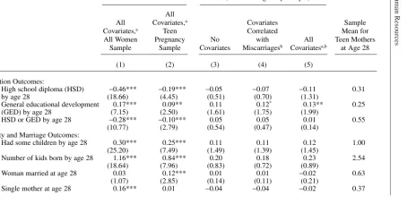
Table 3 presents estimates of the impact of teenage childbearing at age 28 using alter-native samples and methods. Column 1 contains estimates of the effects of not delay-ing childbeardelay-ing until adulthood usdelay-ing OLS methods, controlldelay-ing for background characteristics, on the All Women sample; Column 2 contains OLS estimates with the same controls as Column 1, using the Teen Pregnancy sample; Column 3 contains IV estimates with no controls; Column 4 are IV estimates with controls for the covariates correlated with nonrandom miscarriages; and Column 5 shows the IV estimates that include a full set of control variables, that is, background characteristics and corre-lates with nonrandom miscarriages. The final three columns are estimated with the Teen Pregnancy sample. We also include a column with the sample means of each of these outcomes for teen mothers when they were age 28.
Consider first the estimates in Column 1 of Table 3. These estimates mirror the methodology used in a number of the previous studies of the effects of teenage child-bearing. (See the Introduction for a partial list of these studies.) Consistent with those findings, the estimates in Column 1 typically indicate “adverse” consequences of women not delaying their childbearing until adulthood on a range of subsequent maternal outcomes. Compared to women who delayed childbearing until after age 18, teen mothers (at age 28) were 46 percent less likely to have received a high school diploma; had 1.16 more children on average; were 16 percent more likely to be a sin-gle mother; had worked 170 fewer hours per year; had lower wages ($.88 per hour lower);23and earned $3,780 less in the paid labor market per year. In addition, teen
mothers (at age 28) were in households with, on average, $2,231 less in spousal
22. Age 28 is the oldest age for which we have year-by-year data on women from all birth cohorts in the NLSY79.
The Journal of Human Resources
Table 3
Change in Outcomes Due to Not Delaying Childbearing Measured at Age 28
OLS IV (on Teen Pregnancy Sample)
All
All Covariates,a Covariates Sample
Covariates,a Teen Correlated Mean for
All Women Pregnancy No with All Teen Mothers
Sample Sample Covariates Miscarriagesb Covariatesa,b at Age 28
(1) (2) (3) (4) (5)
Education Outcomes:
1. High school diploma (HSD) −0.46*** −0.19*** −0.05 −0.07 −0.11 0.31
by age 28 (18.66) (4.45) (0.51) (0.70) (1.31)
2. General educational development 0.17*** 0.09** 0.11 0.12* 0.13** 0.25
(GED) by age 28 (7.15) (2.50) (1.61) (1.75) (1.99)
3. HSD or GED by age 28 −0.28*** −0.10*** 0.05 0.05 0.01 0.55
(10.77) (2.79) (0.54) (0.47) (0.14)
Fertility and Marriage Outcomes:
4. Had some children by age 28 0.30*** 0.25*** 0.11 0.11 0.12 1.00
(25.20) (7.49) (1.49) (1.39) (1.45)
5. Number of kids born by age 28 1.16*** 0.84*** 0.20 0.18 0.23 2.54
(18.64) (7.96) (0.83) (0.72) (0.89)
6. Woman married at age 28 0.03 0.12*** 0.01 0.01 −0.02 0.63
(1.07) (2.85) (0.14) (0.11) (0.21)
Hotz, McElro
y, and Sanders
697
8. Annual hours worked at age 28 −170*** −21 405** 420** 317* 1,039
(2.96) (0.24) (2.26) (2.24) (1.67)
9. Cumulative number of hours −2,009*** −969 2,600** 2,790** 2,031 7,759
worked by age 28 (5.19) (1.56) (2.24) (2.36) (1.49)
10. Hourly wage rate at age 28 −0.88** −0.91 1.82 2.07* 2.72** 7.90
(in 1994$)c (2.03) (1.42) (1.53) (1.65) (2.07)
Earnings-Related outcomes:
11. Woman’s annual earnings at −3,780*** −2,599*** 4,677*** 5,075*** 4,218** $7,500
age 28 (in 1994$) (3.50) (2.68) (2.93) (2.95) (2.47)
12. Annual earnings of spouse at −2,213** 115 1,177 1,029 1,668 $10,742
age 28 (in 1994$) (2.07) (0.06) (0.31) (0.28) (0.45)
13. Fraction living in poverty at 0.15*** 0.06 −0.14 −0.14 −0.13 0.47
age 28 (5.36) (1.42) (1.40) (1.43) (1.41)
Public Assistance Outcomes:
14. On AFDC while age 28 0.11*** 0.02 −0.05 −0.06 −0.02 0.27
(4.85) (0.57) (0.62) (0.65) (0.21)
15. Received food stamps while 0.14*** 0.04 −0.07 −0.07 −0.03 0.36
age 28 (5.76) (1.07) (0.81) (0.82) (0.33)
16. Annual public assistant benefits 1,159*** 230 −510 −455 53 $2,787
at age 28 (in 1994$) (4.84) (0.69) (0.57) (0.53) (0.07)
Notes: Dollar figures in 1994 dollars. Robust t-statistics in parentheses. Estimates derived from weighted regressions.
a. Regression includes dummy variables for the woman’s age as of 1979, ethnicity (black and Hispanic), living in a female-headed family at age 14, living in an intact fam-ily at age 14, and whether woman’s AFQT score fell in 1st, 2nd, or 3rd quartiles of distribution, as well as measures of woman’s famfam-ily income in 1978 (in 1994$), her mother’s and father’s educational attainment, and missing value indicators for the last three variables.
income; were 15 percent more likely to reside in a household with total income below the poverty level; were more likely to receive public assistance; and received $1,159 more from these programs. Furthermore, most of these estimated effects are sizeable relative to the average outcomes for teen mothers in our data. For example, these esti-mates imply that fraction of teen mothers receiving high school diplomas would have been 1.5 times higher and would have had 50 percent higher earnings at age 28 if they had delayed their childbearing.24If such estimates accurately characterize the causal
effects of teenage childbearing, they imply that the failure of teen mothers to delay their childbearing has dire consequences for the socioeconomic attainment of these women that are sizeable and apparently persistent.
As one moves across the columns in Table 3, changing the sample used and exploiting the “miscarriages-as-a-natural-experiment” in the estimation of the effects of teenage childbearing, we find that the adverse effects found in Column 1 are pro-gressively weakened and, for some outcomes, are even reversed. Furthermore, the estimates in the subsequent columns suggest a very different set of conclusions about the consequences of early childbearing for teenage mothers. Simply changing the sample from All Women to those who were pregnant as teens, Column 1 versus Column 2, we find that the adverse effects of teenage childbearing appear to be reduced, after controlling for a comparable set of covariates. For some outcomes, such as single motherhood (Row 7), all of the work-related outcomes (Rows 8–10), spousal income (Row 12), and the public assistance measures (Rows 14–16), the estimated effects are no longer statistically significant and the effects on being mar-ried actually reverse sign and are statistically significant compared to the OLS esti-mates in Column 1. Thus, it does appear that using a more comparable comparison group, namely women who become pregnant as teens but do not have a teen birth, to estimate the counterfactual outcomes for teen mothers does alter one’s inferences about the effects of early childbearing.
A comparison of either Column 2 or 1 with the IV estimates in Columns 3 through 5 of Table 3 clearly demonstrates that using miscarriages as an instrument has even more dramatic consequences for the estimation of the causal effects of teenage child-bearing. All of the IV estimates, except for the effects on obtaining a GED, are either statistically insignificant or are significant and have the opposite sign of the OLS esti-mates. Note that for most of the outcomes in Columns 3 through 5 in Table 3 the IV estimates—and the inferences they imply about the effects of teenage childbearing— are quire similar. Among the statistically significant IV estimates, we find that a teen mother’s annual hours of work are between 317 and 420 higherand her annual earn-ings are between $4,218 and $5,075 higherat age 28 than if she had delayed her childbearing. Furthermore, these effects are sizeable. If teen mothers had delayed their childbearing, their annual hours of work and annual earnings would have been, respectively, 30 to 40 percent and 56 to 62 percent lowerat this age relative to the
average values of these outcomes for teen mothers. In short, which samples and, more importantly, what statistical methods one uses has a profound impact on the infer-ences one draws about the consequinfer-ences of teenage childbearing for the socioeco-nomic attainment of this group of women.
B. IV Estimates on Maternal Outcomes over Life Cycle
We now turn to a more detailed consideration of our estimated effects for particular outcomes and examine how these effects vary over the life cycle. IV estimates—with and without covariates and organized by types of outcomes at each age, 18 through 35—are presented in Tables 4 through 7.25We focus on whether and how the effects
of teenage childbearing vary over the life cycle. Having children when women are teenagers, rather than delaying them, is a decision about the timingof fertility. Much of the previous literature has suggested that this timing decision has permanent (and adverse) consequences, for example, higher completed fertility or less success in both labor and marriage markets. Alternatively, the timing decision may have rather tran-sitory consequences for some or all of a teen mother’s subsequent life. We present evi-dence below on which of these alternatives better characterizes the consequences of teenage childbearing.
1. Educational Attainment
We begin with the effects of teenage childbearing on a women’s subsequent educa-tional attainment. Since there is little change in the educaeduca-tional attainment of the women in either of our samples after the early twenties, we restrict our attention to attainment by age 28, as displayed in the first three rows of Table 3. While previous studies and our OLS estimates suggest that teenage childbearing has negative effects on educational attainment, we find little evidence of this in our IV estimates. While negative, our IV estimates of the effect of teenage childbearing on having attained a regular high school diploma by age 28 in Columns 3 through 5 are always small, vary-ing between a 5 to 12 percentage-point decrease in the likelihood of havvary-ing attained a high school diploma and are never statistically significant. In contrast, teenage childbearing appears to increasethe rate of completion of the General Educational
The Journal of Human Resources Table 4
Estimates of the Effect of Teenage Childbearing on Fertility and Marriage Outcomes
Had Some Children Number of Kids Born Woman Married Single Mother
by Age a as of Age a at Age a at Age a
Age of No All No All No All No All
Mother Covariates Covariates Covariates Covariates Covariates Covariates Covariates Covariates
18 0.56*** 0.61*** 0.63*** 0.71*** 0.09 0.09 0.28*** 0.33***
(6.12) (7.03) (4.64) (5.98) (0.71) (0.69) (3.22) (4.25)
19 0.43*** 0.48*** 0.66*** 0.73*** 0.02 −0.01 0.19** 0.24***
(4.52) (5.06) (4.77) (6.01) (0.22) (0.05) (2.23) (2.99)
20 0.28*** 0.31*** 0.47*** 0.60*** 0.05 0.03 0.06 0.10
(3.04) (3.35) (2.66) (4.12) (0.55) (0.34) (0.75) (1.16)
21 0.19** 0.21** 0.42** 0.57*** 0.06 0.04 0.00 0.03
(2.11) (2.28) (2.11) (3.61) (0.67) (0.41) (0.02) (0.31)
22 0.21** 0.23** 0.42** 0.55*** 0.03 0.01 −0.01 0.01
(2.36) (2.53) (1.99) (3.13) (0.31) (0.06) (0.14) (0.12)
23 0.15* 0.17* 0.36* 0.46** 0.06 0.04 −0.07 −0.06
(1.82) (1.93) (1.67) (2.49) (0.57) (0.41) (0.75) (0.62)
24 0.17** 0.19** 0.33 0.43** 0.04 0.02 −0.04 −0.02
(2.04) (2.11) (1.48) (2.09) (0.46) (0.21) (0.38) (0.25)
25 0.16* 0.17** 0.32 0.40* −0.02 −0.05 0.02 0.04
(1.91) (1.97) (1.36) (1.79) (0.17) (0.56) (0.22) (0.51)
26 0.14* 0.15* 0.25 0.32 0.05 0.02 −0.03 −0.02
(1.76) (1.79) (1.07) (1.38) (0.54) (0.24) (0.37) (0.18)
27 0.14* 0.15* 0.19 0.24 −0.04 −0.07 0.04 0.06
Hotz, McElro
y, and Sanders
701
29 0.11 0.13 0.21 0.30 0.02 0.01 −0.08 −0.06
(1.35) (1.55) (0.81) (1.17) (0.23) (0.12) (0.77) (0.61)
30 0.10 0.12 0.22 0.29 0.10 0.08 −0.14 −0.13
(1.27) (1.39) (0.77) (0.99) (0.88) (0.80) (1.32) (1.29)
31 0.10 0.12 0.29 0.32 0.12 0.09 −0.16 −0.13
(1.21) (1.31) (0.98) (1.06) (1.01) (0.87) (1.36) (1.26)
32 0.13 0.14 0.62** 0.53 0.07 0.09 −0.10 −0.13
(1.34) (1.36) (2.00) (1.56) (0.57) (0.85) (0.82) (1.16)
33 0.16 0.18 0.55 0.48 −0.08 −0.03 0.05 0.00
(1.20) (1.32) (1.39) (1.11) (0.61) (0.31) (0.36) (0.04)
34 0.22 0.23 0.60 0.62 0.00 −0.05 −0.02 0.02
(1.32) (1.43) (1.15) (1.22) (0.02) (0.37) (0.15) (0.17)
35 0.50* 0.51** 1.71** 1.71*** 0.11 0.09 −0.11 −0.08
(1.88) (2.09) (2.42) (2.60) (0.41) (0.39) (0.41) (0.31)
Number of
person-ages 14,839 14,096 14,839 14,096 14,428 13,716 14,428 13,716
Development (GED) certificate,26by between 11 to 13 percentage points, and the IV estimates that control for covariates are statistically significant at modest levels. Thus, it appears that teen mothers compensate for their lower rates of attaining a high school diploma by receiving a GED. However, this substitution is only partial. We find no statistically significant effect of early childbearing on the probability that teen moth-ers obtain a high school level education—either in the form of a regular high school diploma or GED—relative to what would have happened to these women if they had delayed their childbearing.
It is unclear what the implications are of this apparent substitution by teen mothers of attaining a GED rather than a regular high school diploma. Cameron and Heckman (1993) find that the value of the GED in the labor market is minimal, with its recipi-ents earning no more than high school dropouts. If their findings apply to teen moth-ers, the consequences of this substitution of a diploma for a GED are not innocuous, at least not for labor market earnings. However, the Cameron and Heckman analysis is only for men. In a subsequent study of the GED for womenCao, Stromsdorfer and Weeks (1996) find that the labor market returns (in terms of earnings) to a GED are no different from the returns to a high school diploma. What remains to be determined is whether this result also holds for the subset of women who become teen mothers.
2. Fertility and Marriage
In Table 4, we present age-specific IV estimates of the causal effects of teenage child-bearing on women’s subsequent fertility and marriage outcomes. We consider the effects of teenage motherhood on the number of children to whom a woman gives birth and on the probability of having any children at each age. Since according to our definition of teen mothers, all teen mothers have children by age 18, it is important to recognize that the estimated effects of a woman not delaying her childbearing until adulthood (that is, age 18 and older) on her subsequent fertility are measured relative to what would have happened if she had delayed her fertility. That is, the counterfac-tual outcome here is the life cycle childbearing pattern of fertility for “latent-birth” women characterized in Section III, where we use miscarriages to estimate their out-comes. While the latent-birth (hypothetical) women, by definition, delay their child-bearing, at issue is how long they delay their childbearing. The estimates in the first two sets of columns in Table 4 indicate that, on average, they do not delay childbear-ing much past their early twenties and, in many cases, for even less time than that.
According to the estimates in the first column of Table 4, only 56 percent of latent-birth type women have not had a child by age 18.27Regardless of the IV estimates used, by age 24, only between 17 and 19 percent of latent-birth type women have not had a child, with these rates of “no birth” diminishing further with age. The estimated effects actually start to rise when women reach age 30 and older, although, as noted above, these estimates are based on much smaller numbers of observations. Because
26. The GED is granted upon the successful completion of an examination that tests competency in a basic high school curriculum. The GED does not require a fixed class schedule and may offer teenage mothers sub-stantial flexibility in study time.
of the generally high fertility among latent-birth women, the effect of teenage child-bearing on the number of children to whom a woman gives birth is never more then 0.84 and declines to 0.30 in her late 20s. A similar age pattern holds for the estimated effects of teenage childbearing on the number of children born by the time the woman reaches various ages (see Table 4). Thus, while teenage childbearing does clearly increase the incidence of births and family size in the short run relative to the coun-terfactual state of postponing childbearing until they are older, this effect fades rather quickly with age. Thus, as seen in Table 3, the effect of not postponing childbearing by teen mothers is negligible and insignificant by age 28.
Table 4 also presents IV estimates of the effects of teenage childbearing on whether a woman is married and is a single mother at age a,which combines information on a woman’s marital and fertility statuses. As is clear from Table 4, the effects of early childbearing on the likelihood of being married (regardless of a woman’s fertility sta-tus) are small and always statistically insignificant. We find that at ages 18 and 19, being a teenage mother increases the chances of being a single mother by 28 percentage points and 19 percentage points, respectively but no significant effect is found at older ages. In fact, the estimated effects at older ages tend to be negative, although none of them is statistically significant. Thus, the effects of teenage childbearing on single motherhood are even more transitory than the effects on fertility alone, with the early effects driven almost entirely by the higher rates of motherhood at early ages.
3. Hours of Work and Wages
Table 5 displays IV estimates of the effects of early childbearing on annual hours of work, cumulative number of hours worked, and hourly wage rates at different ages over a woman’s life cycle. Consider the effects on annual hours of work in the first set of columns in this table. While women who have teen births work slightly fewer hours at ages 18 and 19 than they would have if they had delayed their childbear-ing, from age 20 on, they actually work more hours in a year than if they had post-poned their childbearing. By age 28, for example, women who have their first births early work between 342 and 405 more hours than if they had delayed their child-bearing until adulthood. Some of these differences are statistically significant when teen mothers are in their mid to late twenties, although the age-specific estimates that control for covariates are less precisely estimated. Finally, we note that these estimated effects are not trivial in magnitude. Over the ages of 21 through 35, teen mothers worked an average of 1,045 hours per year. Based on the “All Covariates” estimates, teen mothers would have worked an average of 21 percent fewer hours per year over this age range if they had delayed their first birth until adulthood. Moreover, the negative effects of not delaying childbearing as a percentage of hours of work become larger with age, rising to 29 percent fewer hours when teen moth-ers are in their early thirties.
The Journal of Human Resources Table 5
Estimates of the Effect of Teenage Childbearing on Work and Wage Outcomes
Woman’s Ann Hours Cumulative Number of Hourly Wage Rate
Worked at Age a Hours Worked at Age a at Age a
No All No All No All
Age of Mother Covariates Covariates Covariates Covariates Covariates Covariates
18 −68 −140 114 −214 −$2.93 −$4.45
(0.47) (0.76) (0.53) (0.33) (1.03) (1.44)
19 −145 −239 −66 −349 $1.26 $0.82
(0.96) (1.62) (0.22) (0.62) (1.61) (0.86)
20 251* 193 313 181 $0.45 $0.17
(1.74) (1.30) (0.96) (0.38) (0.40) (0.14)
21 186 145 352 231 $1.28 $0.81
(1.17) (0.80) (0.99) (0.45) (0.95) (0.58)
22 147 37 639 181 −$0.40 −$0.84
(0.96) (0.22) (1.42) (0.31) (0.34) (0.71)
23 76 −7 883* 444 −$1.44 −$1.87
(0.45) (0.04) (1.66) (0.69) (0.93) (1.19)
24 215 118 954 360 $1.34 $0.93
(1.18) (0.60) (1.43) (0.48) (1.38) (0.92)
25 331* 254 1,160 701 $0.75 $0.26
(1.91) (1.33) (1.43) (0.76) (0.51) (0.19)
26 374** 306 1,424 949 −$1.49 −$2.06
(2.20) (1.60) (1.54) (0.92) (0.49) (0.69)
27 344* 285 1,963* 1,186 $2.19 $1.93
Hotz, McElro
y, and Sanders
705
29 70 −47 1,747 1,120 $1.08 $2.29
(0.30) (0.18) (1.28) (0.79) (0.48) (1.45)
30 106 96 2,097 1,559 $2.73** $2.11*
(0.47) (0.40) (1.31) (0.90) (2.10) (1.76)
31 230 329 994 368 −$7.86 −$9.07
(0.94) (1.39) (0.52) (0.18) (1.14) (1.26)
32 479** 511** 355 −31 $1.00 $0.11
(1.97) (1.99) (0.16) (0.01) (0.58) (0.07)
33 470 556 2,398 1,848 $2.44 $0.86
(1.51) (1.48) (0.83) (0.60) (1.09) (0.50)
34 494 542 1,662 2,251 $0.55 $0.56
(1.55) (1.51) (0.54) (0.65) (0.25) (0.26)
35 −131 −129 −3,567 −3,338 $2.59 $2.46
(0.41) (0.38) (0.76) (0.67) (0.77) (0.82)
Number of person-ages 13,508 12,907 13,508 12,907 8,045 7,785
The Journal of Human Resources Table 6
Estimates of the Effect of Teenage Childbearing on Earnings-Related Outcomes
Woman’s Annual Earnings Annual Earnings of Spouse Living in Poverty
at Age a at Age a at Age a
No All No All No All
Age of Mother Covariates Covariates Covariates Covariates Covariates Covariates
18 −$360 −$1,240 $3,744*** $2,054 −0.06 −0.03
(0.30) (0.70) (2.76) (0.89) (0.67) (0.31)
19 −$759 −$1,706 $2,956* $878 0.04 0.06
(0.58) (1.03) (1.94) (0.43) (0.40) (0.59)
20 $1,665 $1,312 $3,681** $3,337* −0.12 −0.13
(1.61) (1.05) (2.39) (1.87) (1.27) (1.30)
21 $2,435** $2,108 $1,624 −$177 −0.04 −0.04
(2.22) (1.49) (0.65) (0.07) (0.43) (0.45)
22 $1,092 $191 $3,082 $2,297 −0.03 −0.03
(0.89) (0.15) (1.29) (0.97) (0.34) (0.37)
23 $806 $42 $1,207 $746 0.02 0.03
(0.51) (0.02) (0.44) (0.26) (0.18) (0.27)
24 $2,792* $2,072 $4,692* $3,780 −0.05 −0.04
(1.93) (1.27) (1.77) (1.43) (0.47) (0.48)
25 $3,174** $2,542 $4,683 $3,962 −0.11 −0.12
(2.16) (1.59) (1.64) (1.38) (1.12) (1.21)
26 $3,812** $3,213* $2,713 $2,523 −0.07 −0.08
(2.44) (1.87) (0.89) (0.86) (0.71) (0.83)
27 $4,530*** $4,210** $2,361 $2,126 −0.09 −0.10
Hotz, McElro
y, and Sanders
707
29 $3,075 $2,327 $8,198*** $7,349*** −0.07 −0.06
(1.61) (1.21) (3.28) (2.92) (0.73) (0.67)
30 $3,634* $2,959 $5,434* $5,922** −0.08 −0.09
(1.76) (1.46) (1.88) (2.18) (0.76) (0.89)
31 $1,439 $1,021 $8,923** $11,029*** −0.16 −0.19*
(0.65) (0.45) (2.39) (4.12) (1.37) (1.71)
32 $2,875 $2,938 $5,055 $7,939*** 0.00 −0.07
(1.02) (1.00) (1.23) (2.65) (0.03) (0.54)
33 $4,496 $4,848 $4,719 $7,932** −0.12 −0.23*
(1.37) (1.40) (1.06) (2.29) (0.74) (1.71)
34 $3,632 $4,511 $15,923*** $15,545*** −0.28* −0.27*
(0.96) (1.13) (3.89) (3.66) (1.78) (1.81)
35 $435 $861 $8,093 $8,516 −0.21 −0.21
(0.07) (0.16) (1.55) (1.58) (0.85) (0.90)
Number of person-ages 13,396 12,804 13,272 12,665 14,839 14,096
those for the other socioeconomic outcomes we consider in this article. Note that wage rates are measured only at ages when women work and our estimation strategy does not account for this source of selectivity. Without further assuming that our instrumental variable (IV) is uncorrelated with whether a woman works—an assump-tion that is not readily justifiable—our IV estimator of the effects of early childbear-ing on wages need not be consistent. Thus, the estimates in Table 5 for wages—as well as the corresponding estimates in Table 3—do not have the same credibility as to those for the other outcomes we consider and should be interpreted with much greater caution. With this important caveat, we briefly consider the estimated effects of teenage childbearing on a woman’s hourly wages. Unlike annual hours of work, there is little evidence of a strong life cycle pattern with respect to the effects of early child-bearing on hourly wage rates based on the age-specific estimates presented in Table 5. Furthermore, with the exception of age 30, the age-specific estimates of these effects are not precisely estimated. Thus, we tentatively conclude that early childbearing does not result in permanently lower wage rates relative to what teen mothers would have received if they had delayed their childbearing.
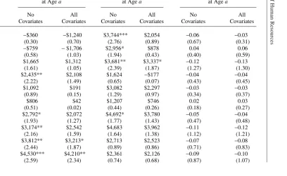
4. Earnings and the Incidence of Living in Poverty
In Table 6, we examine the effect for teen mothers of not delaying their childbearing on their labor market earnings, spousal earnings, and the likelihood that they live in poverty. As shown in Table 5, not delaying their births actually resulted in increased hours of work when these women reached their mid- to late twenties and did not result in any significant declines in the wages they received. Thus, our finding that not delaying childbearing led to an increase in the labor market earnings of these women starting at ages 24 or 25 is plausible rather than surprising (refer to the first two columns of Table 6). These effects on a woman’s earnings persist into the thir-ties, although the latter effects for the thirties are not as precisely estimated, possi-bly because of the reduced numbers of observations at these ages. Furthermore, the magnitudes of these estimated effects of teenage childbearing on subsequent labor market earnings are sizeable. Over the ages of 21 through 35, teen mothers earned an average $7,917 per year (in 1994 dollars). Based on the “All Covariates” estimates in Table 6, teen mothers would have earned an average of 31 percent lessper year if they had delayed their childbearing, where the largest reductions are estimated to be 24 percent during the early twenties, 43 percent during the late twenties and 27 per-cent during the early thirties.
Our findings for the life-cycle consequences of teen mothers not delaying their childbearing for their success in the labor market, especially earnings, are in sharp contrast to all previous studies of the effects of teenage childbearing and to the view that teenage childbearing severely restricts the ability of these women to be success-ful in the labor market. While a coherent explanation of why teen mothers appear to benefit from not delaying their childbearing when it comes to the labor market awaits further research, we offer the following speculation.
suggests that these women are more likely to acquire their skills on the job (rather than in school) and work in jobs where educational credentials are less important than continuity and job-specific experience. For such women, concentrating their child-bearing at early ages may prove to be more compatible with their labor market career options than postponing their childbearing to older ages would be. If this characteri-zation is accurate, forcing teen mothers to postpone their childbearing, as miscar-riages do, may “explain” why they both appear to acquire no more formal education and actually end up doing less well in the labor market than if they had been able to follow their preferred life cycle plan.
Estimates of the effects of teen mothers not delaying their childbearing on the financial support they receive in the form of spousal income also are displayed in Table 6. Based on these estimates, there is no evidence that teenage mothers draw sub-stantially less support from spouses over their early to mid-adult years. In fact, start-ing at around age 30, both of the IV estimates presented in the second and third columns of Table 6 indicate that teenage mothers actually derive substantially more support in the form of spousal income than they would have received if they had delayed childbearing.28We have no ready explanation for this finding. We speculate
that it may be related to our finding that teenage mothers are more successful in the labor force, that is, they generate higher earnings, than if they had postponed their childbearing and that this success affects their success in the marriage market, at least with respect to the earnings capacity of a spouse.
Finally, we consider what effects delaying early childbearing would have for the likelihood that teen mothers are in households with such low levels of earnings— from both their own earnings and the earnings of spouses—that they fall below the federal poverty line. IV estimates of the effects of teenage childbearing on the inci-dence of living in poverty are presented in the last two columns of Table 6. Given the results for own and spousal earnings presented in this table, it is not surprising that teenage childbearing does not seem to be associated with an increase in the incidence of living in poverty among teen mothers, in either the short run or the long run. In fact, our estimates suggest that not delaying childbearing actually
reducesthe incidence of poverty, although these effects are statistically significant at only a few older ages. At the same time, a sizeable fraction of women who begin their childbearing as teens (38 percent) do live in poverty during their twenties and early thirties. Our estimates indicate that the incidence of poverty for women who began their childbearing as teens would have been 0.58 times morelikely to live in poverty over this period of their lives if they delayed their childbearing until adulthood.
5. Receipt of Public Assistance
In Table 7, we present estimates of the effects of teenage childbearing on the use of and financial support from several forms of public assistance for ages 18 through 35. In particular, we examine the effects on the following outcomes: (1) whether a woman was receiving public assistance through the Aid to Families with Dependent Children
The Journal of Human Resources Table 7
Estimates of the Effect of Teenage Childbearing on Public Assistance Outcomes
On AFDC while On Food Stamps Annual Public Assistance
Age a while Age a Benefits at Age a
No All No All No All
Age of Mother Covariates Covariates Covariates Covariates Covariates Covariates
18 0.001 0.001 0.06 0.02 $1,048 $1,430*
(0.01) (0.02) (0.57) (0.17) (1.43) (1.80)
19 0.02 0.05 0.11 0.10 $1,101 $1,755***
(0.19) (0.54) (1.16) (1.08) (1.41) (2.66)
20 0.03 0.08 0.04 0.05 $879 $1,441***
(0.31) (0.98) (0.48) (0.51) (1.24) (2.69)
21 −0.04 0.01 0.05 0.06 $603 $1,246**
(0.46) (0.12) (0.57) (0.67) (0.77) (2.24)
22 −0.04 0.01 0.07 0.08 −$94 $600
(0.45) (0.07) (0.89) (0.91) (0.10) (0.81)
23 −0.11 −0.07 −0.12 −0.09 −$293 $276
(1.23) (0.81) (1.29) (0.96) (0.33) (0.42)
24 −0.07 −0.02 −0.11 −0.08 −$715 −$258
(0.73) (0.27) (1.19) (0.85) (0.61) (0.25)
25 −0.09 −0.05 −0.21** −0.18* −$548 −$73
(1.01) (0.57) (2.13) (1.84) (0.56) (0.08)
26 0.03 0.06 −0.22** −0.20** −$83 $123
(0.31) (0.76) (2.18) (2.13) (0.09) (0.14)
27 0.06 0.09 −0.14 −0.12 −$394 $111
Hotz, McElro
y, and Sanders
711
29 −0.09 −0.07 −0.11 −0.10 −$1,174 −$579
(1.02) (0.81) (1.17) (1.08) (1.05) (0.67)
30 −0.07 −0.05 −0.11 −0.11 −$892 −$576
(0.76) (0.65) (1.06) (1.11) (0.73) (0.58)
31 −0.14 −0.13 −0.16 −0.16 −$2,595* −$2,298
(1.37) (1.24) (1.38) (1.35) (1.74) (1.60)
32 −0.06 −0.09 −0.10 −0.16 −$2,684 −$3,323
(0.55) (0.90) (0.81) (1.18) (1.33) (1.63)
33 −0.05 −0.09 −0.02 −0.07 $88 −$461
(0.45) (0.79) (0.15) (0.53) (0.09) (0.45)
34 −0.05 −0.03 −0.07 −0.05 −$598 −$357
(0.46) (0.33) (0.46) (0.41) (0.45) (0.30)
35 −0.04 −0.05 0.09 0.08 −$2,028 −$2,079
(0.27) (0.40) (0.60) (0.55) (0.65) (0.75)
Number of person-ages 14,839 14,096 14,839 14,096 14,235 13,563
(AFDC) program at a particular age a,29(2) whether she received Food Stamps at
that age, and (3) the annual dollar amount (in 1994 dollars) of benefits a woman received from the AFDC, Food Stamps programs and the Medicaid program.30Both
sets of IV estimates of the effects of not delaying births among teen mothers have sim-ilar age patterns for all three of these measures of public assistance. In particular, all three outcomes show that at young adult ages, from age 18 until around 22, the esti-mated effects of teenage childbearing are positive, indicating that teen mothers were more likely to be on public assistance and receive larger amounts of transfers from these programs than if they had delayed their childbearing. For these younger ages, the estimated effects are statistically significant only for the annual amount of bene-fits received in the form of public assistance. However, from around age 22, the esti-mated effects reverse in sign, implying that teen mothers actually reduced their participation in and amount of benefits received from these public assistance pro-grams compared to what they would have done if they had delayed their childbearing. Most of these estimated effects at older ages are not statistically significant, although we do find significant effects for receiving Food Stamps at age 25 and 26. Once again, our IV estimates indicate that the causal effect of teen motherhood does not appear to increase the utilization of various forms of public assistance as suggested by earlier studies.
V. Conclusion
In this study, we have used an alternative and innovative strategy to estimate the causal effects associated with teenage childbearing in the United States. In particular, we have focused on women who first become pregnant as teenagers and employ a natural experiment to obtain a more comparable, and plausible, compari-son group with which to derive estimates of counterfactual outcomes for teen moth-ers. Our results suggest that much of the “concern” that has been registered regarding
29. The Aid to Families with Dependent Children (AFDC) program, a federal program, was replaced in 1996 with the Temporary Assistance for Needy Families (TANF) program.
30. The annual benefits received from AFDC and Food Stamps were derived from women’s responses to annual questions about number of months in a (calendar) year that they were on each of these programs and the average monthly payment/benefit they received. To estimate the implied Medicaid benefits she received, we used the following strategy to estimate the relationship between AFDC and Food Stamps and Medicaid expenditures. In particular, we regressed aggregate state Medicaid expenditures on the sum of aggregate AFDC and Food Stamp expenditures by state, yielding the following regression:
Medicaid Expend. = 250 +0.193(AFDC Expend. +Food Stamp Expend.)
using 1993 monthly data taken from the Green Book(U.S. House of Representatives, Ways and Means Committee, 1994). We interpreted the intercept as being the fixed costs of running a state’s Medicaid pro-gram plusthe expenditures going to non-AFDC/Food Stamp recipients (that is, the Elderly) and calculated the “marginal” Medicaid expenditures for a woman in our sample as:
Medicaid Payments = 0.193(AFDC Expend. +Food Stamp Expend.)