Transitions from Relative Equilibria
to Relative Periodic Orbits
Claudia Wulff
Received: June 1, 1998 Revised: February 8, 2000
Communicated by Bernold Fiedler
Abstract. We consider G-equivariant semilinear parabolic equa-tions whereGis a finite-dimensional possibly non-compact symmetry group. We treat periodic forcing of relative equilibria and resonant periodic forcing of relative periodic orbits as well as Hopf bifurcation from relative equilibria to relative periodic orbits using Lyapunov-Schmidt reduction. Our main interest are drift phenomena caused by resonance. In comparison to a center manifold approach Lyapunov-Schmidt reduction is technically easier. We discuss impacts of our results on spiral wave dynamics.
2000 Mathematics Subject Classification: 35B32, 35K57, 57S20. Keywords and Phrases: spiral waves, equivariant dynamical systems, noncompact groups.
1 Introduction
1.1 Spiral wave dynamics
Relative equilibria and relative periodic solutions are ubiquitous in systems with continuous symmetry. Examples of relative equilibria and relative periodic solutions are spiral waves. Spiral waves have been observed in various chemical and biological systems, for example in the Belousov-Zhabotinsky reaction [5], [26], [35], and in catalysis on platinum surfaces [16].
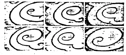
Figure 1: Meandering spiral wave in the Belousov Zhabotinsky reaction, from Steinbock et al. [27], with kind permission of Nature. The tip trajectory is overlaid with a white curve.
a corotating frame. In this case the spiral tip performs a quasiperiodic motion, which is called meandering, see Fig. 1.
Meandering spiral waves are generated by external periodic forcing of rigidly rotating spiral waves [16]. Let ωext be the frequency of the external forcing and let µext be its amplitude. If the periodic forcing is resonant, i.e., if the rotation frequency ω∗
rot of the rigidly rotating wave at µext = 0 is a multiple of the external frequency ωext of the system then a curve of drifting spiral waves in the (ωext, µext)-plane is observed which separates modulated rotating wave states with inward petals and outward petals, cf. [16]. This phenomenon is called resonance drift. Drifting spiral waves, see Fig. 2, are modulated
travelling waves, i.e., they are periodic in a comoving frame. Both, meandering and drifting spiral waves are examples of relative periodic orbits.
In experiments also meandering spiral waves have been forced periodically [35]. Here invariant 3-tori are found and frequency locking between the period of the relative periodic orbits and the period of the external forcing occurs. Further-more for certain external periods modulated travelling waves are generated. Experimentalists call this phenomenon generalized resonance drift [35].
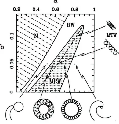
Figure 3: Phase diagram for the spiral wave dynamics depending on the param-eters a,b; courtesy of Barkley [4]. Shown are regions containing N: no spiral waves, RW: stable rigidly rotating waves, MRW: modulated rotating waves, MTW: modulated travelling waves (dashed curve). Spiral tip paths illustrate states at 6 points. Small portions of spiral waves are shown for the two rotating wave cases.
Meandering spiral waves can also emanate from rigidly rotating spiral waves by a spontaneous bifurcation in autonomous systems, see [26], [32]. Barkley found in numerical simulations [3], see Fig. 3, that this transition is a Hopf bifurcation in the corotating frame. Hopf-bifurcation in autonomous systems leads to analogous drifting phenomena as periodic forcing of rigidly rotating waves.
The media in which spiral waves occur can be modelled by reaction-diffusion systems of the form
∂ui
Here u = (u1, . . . , uM) is a vector of concentrations of chemical species, the
functions ui, i = 1, . . . , M, map the plane R2 to R, the constants δi ≥ 0,
i= 1, . . . , M, are diffusion coefficients,µ∈Rpis a parameter, and the functions
fi, i = 1, . . . , M, are reaction-terms which are autonomous or time-periodic.
Barkley [4] was the first to notice the importance of the Euclidean symmetry for spiral wave dynamics. The Euclidean group E(2) = O(2)⋉ R2of rotations, translations and reflections on the plane acts on the functions u(x), x ∈ R2, via
(ρ(R,a)u)(x) =u(R−1(x−a)), where R∈O(2), a∈R2. (1.2) System (1.1) is equivariant with respect to the symmetry group E(2).
In this article we want to study the transition from rigidly rotating to mean-dering spiral waves on the infinitely extended plane R2. More generally the aim of the paper is to understand the transition from relative equilibria to rel-ative periodic orbits in equivariant systems. Furthermore we want to explain the drift and resonance effects which we just described for general symmetry groups. We will discuss implications of our results on spiral wave dynamics in the plane and on the sphere (for simulations of spiral waves on the sphere see [36]). Further we want to apply our results to the evolution of scroll-waves in three-dimensional excitable media. Scroll waves have been studied numerically for example in [15], [18].
1.2 Related literature
In the thesis [33] the first results on bifurcations from rotating waves in systems with a non-compact, non-commutative symmetry group have been obtained. This paper is based on the dissertation [33]; but whereas in [33] we restricted attention to the symmetry group E(2) and applications in spiral wave dynamics in this article we treat arbitrary symmetry groups. As in [33] we study the transition from relative equilibria to relative periodic orbits using Lyapunov-Schmidt reduction.
Shortly after [33] was finished a whole bunch of papers on spiral wave dynamics and non-compact symmetry groups appeared:
Scheel [24], [25] proved the existence of rotating waves in unbounded domains. The thesis [33] was inspired by work of Renardy on bifurcations from rotating waves [19]. Renardy also studied bifurcations from rotating waves of semilinear differential equations using Lyapunov-Schmidt reduction and applied his results to the Laser equations [20]. But his results for partial differential equations are restricted to compact symmetry groups.
1.3 Lyapunov-Schmidt-reduction versus center-manifold theory To analyze bifurcations there are mainly two reduction methods: center-manifold reduction and Lyapunov-Schmidt reduction. Both have advantages and disadvantages. Here we will use Lyapunov-Schmidt reduction as tool for the analysis of bifurcations; for a center-manifold approach see [21], [22]. The advantage of Lyapunov-Schmidt reduction versus center-manifold theory is that we obtainC∞-paths of relative periodic orbits if the nonlinearity in (1.1) isC∞
whereas we only obtain aCk-smooth center-manifold,k <∞. Besides this we
do not need the assumptions that the group action is isometric and that the group orbit of the relative equilibrium is an embedded manifold which are nec-essary for the center-manifold reduction. Finally the proofs are simpler since they do not rely upon the highly developed invariant manifold machinery. On the other hand the Lyapunov-Schmidt method is limited to relative equilibria and relative periodic orbits – we cannot handle more complicated dynamics. But for our purposes this is sufficient.
1.4 Organization of the paper The paper is organized as follows.
1.5 Functional-analytic framework
To describe spiral wave dynamics we consider reaction-diffusion systems of the form (1.1) on a domain Ω ⊂ R3 to R, where Ω is a C∞-manifold without boundary, for exampleR2, the unit sphereS2 inR3 orR3itself. The reaction-termsfi,i= 1, . . . , M, are assumed to be Ck-smooth functions where k∈N.
The domain Ω is invariant under some subgroupGof the Euclidean group E(3) of motions in three-dimensional space consisting of rotations, reflections and translations. The group E(3) = O(3)⋉ R3 acts on the functionsu(x),x∈R3, via (1.2), i.e.,
(ρ(R,a)u)(x) =u(R−1(x−a)), where R∈O(3), a∈R3.
System (1.1) is equivariant with respect to the group G. If G= E(2) is the Euclidean group of motions in the plane we write (φ, a) for (Rφ, a) where Rφ
is a rotation with angleφanda∈R2.
We consider (1.1) in the space of bounded uniformly continuous functionsX=
BCunif(Ω,RM) or in the spaceX =L2(Ω,RM).
InX =BCunif we get a time-evolution Φt,t0 of (1.1) onY =X; ifX=L
2we obtain a time-evolution onY =Xα, α >1/2 without any growth conditions
onf provided thatf(0, t, µ) = 0 for allt,µandδi>0,i= 1, . . . , M. Ifδi= 0
for somei we still obtain a semiflow onX=H2 provided thatf(0, t, µ)≡0. Note that the group action is not smooth on the whole function spaceX. If the domain is Ω = R2 and we choose X = BCunif(R2,RM) then the E(2)-action is even not strongly continuous because on the functionu(x1, x2) = cosx1 the rotation acts discontinuously: For large radiusrthe term|(ρ(φ,0)u)(x)−u(x)| can become equal to 2 even for arbitrarily small φ. We encounter the same problem if Ω =R3. Since we want to have a strongly continuous group action on our base spaceX we consider the reaction-diffusion system (1.1) on a subspace ofBCunif which is invariant under the semiflow and where the group acts in a strongly continuous way:
We defineBCEucl(RN,RM) as the subspace ofBCunif(RN,RM) on which E(N) acts continuously, N = 2,3. The Laplacian is sectorial onX = BCunif and on L2, see [13]. We will now show that the Laplacian is also sectorial on
X =BCEucl(RN,RM): letY be any Banach space with a groupGacting on it by a (not necessarily strongly continuous) representationρg,g∈G. LetY0 be the subspace ofY on whichGacts strongly continuously. IfAis sectorial onY
andAρg=ρgAfor allg∈GthenAis sectorial inY0: fromρge−At= e−Atρgwe
deduce that (e−At)
t≥0 is aC0-semigroup from Y0 to Y0; furthermore e−Aty is complex differentiable intfory∈Y,t >0, with derivativeAe−Aty∈Y. Since
ρgAe−At=Ae−Atρg and therefore Ae−AtY0 ⊂Y0 we conclude that (e−At)t≥0 is an analytic semigroup on Y0. Since (λ−A)−1u ∈ Y0 for u ∈ Y0, λ ∈ C,
We also get a time-evolution of (1.1) in BCEucl(RN,RM) because we have
ρgΦt,t0(u) = Φt,t0(ρgu) and therefore Φt,t0 mapsY0 into itself.
Now we have a C0-group action on X =BCEucl, but if Ω =R2,R3 the semi-flow does not smoothen the group-action even if all diffusion coefficientsδi are
positive. We demonstrate this for Ω =R2and for the heat equation where the nonlinearityf is zero.
We will show that onR2the operator ∂
∂φ is not bounded w.r.t. the Laplacian
∆ and to the semiflow (e∆t) t≥0:
Remark 1.1 The operator ∂
∂φ is not bounded relatively to the Laplacian∆ or
relatively to the semiflow e∆t,t≥0, onBCunif(R2,R)andBCEucl(R2,R). Proof. The functionswℓ,b(x) :=Jℓ(b|x|)eiℓarg(x)whereb≥0 andJℓis theℓ-th
Bessel function of the first kind are elements ofBCEucl(R2,R)⊂BCunif(R2,R) and they are eigenfunctions of the Laplacian ∆ and of the angle derivative ∂
∂φ:
∂
∂φwℓ,b= iℓwℓ,b, ∆wℓ,b=−b
2w
ℓ,b.
Since iℓ(1 +b2)−1 and iℓe−b2t are not bounded for arbitrary b ∈ R, ℓ ∈
N0, we conclude that ∂
∂φ is not bounded relatively to ∆ on BCEucl(R2,R),
BCunif(R2,R) and that ∂φ∂ e∆t is not a bounded operator on BCEucl(R2,R),
BCunif(R2,R) fort≥0.
Remark 1.2 Also on L2(R2,R) the angle-derivative ∂
∂φ is not bounded
rela-tively to ∆ ore∆t,t≥0.
Proof. By direct computation we see that F(∂ ∂φu) =
∂
∂φF(u). Here F(u)
denotes the Fourier transform ofu. From this formula and fromF(∆u)(x) =
−|x|2F(u)(x) we deduce that ∂
∂φ is not bounded with respect to ∆.
Fur-thermore the operator ∂
∂φ is not bounded relatively to e
∆t in L2(R2,R) since (F( ∂
∂φe
∆tu))(x) = ∂ ∂φe
−|x|2t
(F(u))(x) is not defined for allu∈L2(R2,R). Therefore we cannot simply change coordinates into a corotating frame to deal with the meandering transition.
1.6 Representations of E(N)
The function spacesY =BCEucl(RN,R), L2(RN,R),N = 2,3, do not contain finite-dimensional subspaces which are E(N)-invariant and in which the E(N )-action is non-trivial. Again we will demonstrate this in the case Ω = R2,
G= E(2):
Lemma 1.3 Let the action of E(2) on the spaces X = BCEucl(R2,R), X =
L2(R2,R)be given by (1.2). Then the function spaces BCEucl,L2 do not
In Greenleaf [12] a general theory on the action of topological groups on function spaces is developed.
If we allow polynomial growth in our function space then the polynomials of degree≤j are finite-dimensional representations of E(2).
Proof of Lemma 1.3. Let Vj = span(e1, . . . , ej) be a j-dimensional
repre-sentation of E(2) in BCunif or L2. Then the translations act as aC0-group of isometries on Vj since they act in such a way on BCunif, L2. Since Vj is
finite-dimensional, we know that ρ(0,(a1,a2))ei =
Pj
i=1(eη1a1+η2a2)ijej where
η1=∂x∂1|Vj,η2=
∂
∂x2|Vj are (j, j)-matrices. Sinceρ(0,a)is an isometry we con-clude that Re spec(η1) = Re spec(η2) = 0 and thatη1, η2do not contain Jordan blocks. After simultaneous diagonalization of η1, η2 (note that [η1, η2] = 0) we see that the eigenfunctions ofη1,η2 are of the form eibx, b, x∈R2. These functions are not elements of X =L2(R2,R). So the proof is finished for the function spaceL2. If we chooseb= 0 we obtain an E(2)-invariant subspace of
X =BCunif(R2,R) which consists of all constant functions. The E(2)-action on this space is trivial. The action of the rotation is not continuous on the functions eibx, b 6= 0, with respect to the norm k · kBC
unif(R2,R). Therefore
the functions eibx do not span a finite-dimensional E(2)-invariant subspace of
BCEucl(R2,R) forb6= 0.
Of course, the same considerations apply for x ∈ R3, G = E(3) instead of
x∈R2, G= E(2).
Especially for an E(2)-invariant steady state the eigenspace to each eigenvalue is E(2)-invariant and therefore infinite-dimensional. This makes the study of bifurcations from E(2)-invariant equilibria for an abstract equivariant parabolic equation very difficult. We will not attack this problem and rather study bi-furcations from relative equilibria where these difficulties do not occur. Bifur-cations from homogeneous steady states of reaction diffusion equations have been studied by Scheel [24], [25] using spatial dynamics.
1.7 Abstract Setting
In this paper we study semilinear parabolic equations du
dt =−Au+f(u, ωextt, µ) (1.3)
on some Banach space X which are equivariant under a m-dimensional Lie group G which may be non-compact. We assume that A is sectorial (for a definition see [13]) and thatf isCk-smooth fromY×R×RptoX. Herek∈N
or k=∞,µ∈Rp andY =Xα for 0≤α <1.
By [13] there exists a time-evolution Φt,t0(·;µ) of (1.3) onY, and Φt,t0(u;µ) is Ck-smooth in u, µfort≥t0 and inu,µ, t,t0fort > t0. We assume that the groupGacts onY by the linear strongly continuous representationρg∈ L(Y),
g∈Gand that (1.3) isG-equivariant, i.e.,
This implies thatρgΦt,t0(·;µ) = Φt,t0(ρg·;µ) for allg∈G.
Assume thatf in (1.3) is time-independent. Then a group orbitGu∗is called a
relative equilibrium of (1.3) if Φt(u∗) =ρexp(ξ∗t)u∗ for someξ∗∈alg(G). Here alg(G) denotes the Lie algebra ofG. Sometimes we denoteu∗itself as relative
equilibrium.
A pointu∗ lies on arelative periodic orbit
O∗ ={ρgΦt,0(u∗)|g∈G, t∈R}
if ΦT∗,0(u∗) =ρg∗u∗ for some T∗ >0, g∗ ∈G. In this case we suppose that
f(u, ωextt, µ) is independent of time or time-periodic with frequency ωext = 2πj/T∗, j ∈ N. Sometimes we sloppily denote u∗ itself as relative periodic
orbit. We callT∗the relative period of the relative periodic orbit.
The aim of this article is to study transitions from relative equilibria to relative periodic orbits of (1.3).
2 Periodically forcedG-equivariant systems
This section deals with the effects of periodic forcing on relative equilibria and relative periodic orbits. In particular, we will investigate drift phenom-ena caused by resonant periodic forcing. We will apply our results to spiral wave dynamics. This helps to understand the experiments mentioned in the introduction. Proofs of the main theorems are postponed to section 4.
In this section we assume that the nonlinearityf of (1.3) is of the form
f(u, t, µ) = ˆf(u,µˆ) +µextfext(u, ωextt, µ).
Here fext(u, τ, µ) is 2π-periodic in τ; ωext is the frequency of the periodic forcing, Text = ω2extπ is its period, µext is its amplitude and we decompose
µ = (µext,µˆ), where µext ∈ R, ˆµ ∈ Rp−1. So we consider the periodically forced differential equation
du
dt =−Au+ ˆf(u,µˆ) +µextfext(u, ωextt, µ). (2.1)
A typical example of the abstract semilinear differential equation (2.1) is a periodically forced reaction-diffusion system on the domain Ω⊂RN,N = 2,3, cf. (1.1):
∂ui
∂t =δi∆ui+ ˆfi(u,µˆ) +µextfext,i(u, ωextt, µ), i= 1, . . . , M. (2.2)
2.1 Periodic forcing of relative equilibria
Consider system (2.1) without periodic forcing, i.e., at µext = 0. Assume that u∗ is a relative equilibrium of the unforced system for the parameter
ˆ
µ= ˆµ∗= 0. Thenu∗ satisfies
Φt(u∗) =ρetξ∗u∗ for someξ∗ ∈alg(G). Since Φ
t(·) is equivariant andCk-smooth intfor t >0
we conclude that etξ∗
u∗isCk-smooth intfor allt∈R.
We will writeξufor ddtρetξu|t=0. Furthermore denote by Adgξ:=gξg−1= d
dt(gexp(ξt)g −1)
t=0∈alg(G) the adjoint action ofGon alg(G) and by
K={g∈G|ρgu∗=u∗}
the isotropy group of u∗. We assume that K is compact. Let G0 denote the identity component of G. We have ξ∗ ∈ alg(N(K)) where N(K) is the
normalizer of the isotropy groupKofu∗ because forg∈K,t∈R,
ρgρexp(tξ∗)u∗=ρgΦt(u∗) = Φt(ρgu∗) = Φt(u∗) =ρexp(tξ∗)u∗
and therefore gexp(tξ∗)∈exp(tξ∗)K. Similarly the pull-back elementg∗ of a
relative periodic orbitu∗=ρ−1
g∗ΦText,0(u
∗) lies in the normalizer of the isotropy K ofu∗. Actually for a relative equilibrium the drift velocityξ∗ lies in the Lie
algebra of the centralizerZ(K) ofK, which follows from the formulaN(K)0=
K0Z(K)0, see [9].
Since by periodic forcing isotropy is not changed we assume without loss of generality in the whole section thatK={id}. Otherwise we change the space
Y to the fixed point space Fix(K) = {g ∈ G, ρgu∗ = u∗} of K and the
symmetry groupGtoN(K)/K.
Letu∗be a relative equilibrium, i.e.,−Au∗+ ˆf(u∗) =ξ∗u∗, and let L∗=−A+ Dufˆ(u∗)−ξ∗
be the linearization at the relative equilibrium in the comoving frame. Assume that ρgu∗ isC1 in g∈G. We compute that forξ∈alg(G)
L∗ξu∗ = (−A+ D
ufˆ(u∗)−ξ∗)ξu∗
= −ξAu∗+ D
ufˆ(u∗)ξu∗−ξ∗ξu∗
= ξ(−A+ ˆf(u∗))−ξ∗ξu∗
= (ξξ∗−ξ∗ξ)u∗
= [ξ, ξ∗]u∗=−ad
ξ∗u∗.
(2.3)
Here [·,·] denotes the commutator, adξ∗(ξ) = [ξ∗, ξ] and we used that gfˆ(u) = ˆ
f(gu) and therefore Dufˆ(u∗)ξ = ξfˆ(u). From (2.3) we see that L∗ maps
Example 2.1 Let u∗ be a rotating wave of the unforced system (2.1), e.g a
rigidly rotating spiral wave of the reaction-diffusion system (2.2) on Ω = R2 at µext = 0. Then the symmetry group is G= E(2). We write g = (φ, a)∈ SO(2)⋉ R2 = SE(2). Let ξ1 denote the generator of the rotation and ξ2, ξ3 denote the generators of the translation. Then ξ∗ =ω∗
rotξ1 where ωrot∗ is the rotation frequency of the spiral, and we compute
L∗ξ1u∗= 0, L∗(ξ2+ iξ3)u∗=ωrot∗ [ξ2+ iξ3, ξ1]u∗= iωrot∗ (ξ2+ iξ3)u∗. Therefore the linearizationL∗ of the rotating wave in the rotating frame has always eigenvalues on the imaginary axis.
For a relative periodic orbitu∗=ρ−1
g∗ΦT∗,0(u∗) withρgu∗ C1in gwe get
ρ−g∗1DΦT∗,0(u∗)ξu∗= (Ad−g∗1ξ)u
∗, ξ∈alg(G).
If u∗ is a relative equilibrium then the linearization of the time-T-map in the
comoving frameξ∗ is given by
eL∗T =ρ−g∗1DΦT(u
∗)
whereg∗= eT ξ∗ .
For the groups relevant in applications (compact and Euclidean groups) the eigenvalues of the linear maps [ξ,·],ξ∈alg(G), on alg(G) are purely imaginary and similarly the spectrum of the maps Adg,g∈G, on alg(G) lies on the unit
circle. We will restrict our attention to these groups in this article. So we make the overall hypothesis
Overall HypothesisThe spectra of the linear mapsAdg,g∈G, are subsets
of the unit circle {λ∈C; |λ|= 1}.
Therefore in the case of continuous symmetry where alg(G) is nontrivial the linearizationL∗ at a relative equilibrium always has eigenvalues on the
imag-inary axis and similarly the linearization ρ−g∗1DΦT(u
∗) of a relative periodic
orbitu∗=ρ−1
g∗ΦT(u∗) of (2.1) has always center-eigenvalues on the unit circle. Ifu∗is a relative equilibrium fix someT >0. In the case of a relative periodic
orbit takeT =T∗. We need the following assumption on the spectrum:
Hypothesis (S) The set {λ∈ C; |λ| ≥ 1} is a spectral set for the spectrum spec(B∗)of the operator
B∗:=ρ−g∗1DΦT(u
∗)∈ L(Y) (2.4)
(called center-unstable spectral set) with associated spectral projectionP ∈ L(Y)
and the corresponding generalized eigenspace Ecu:=R(P)(the center-unstable
eigenspace) is finite-dimensional.
We will show in Section 4 below that Hypothesis (S) implies that ρgu∗ isCk
in g. LetGu∗ ={ρgu∗; g ∈G} denote the group orbit atu∗. Frequently we
Definition 2.2 We say that a relative periodic orbit or a relative equilibrium
u∗ of (2.1) is non-criticalifρ
gu∗ isC1 ing and if the operator B∗ from (2.4)
satisfies Hypothesis (S) and if the center-eigenspace
Ec =Tu∗Gu∗+ span(∂tΦt(u∗)|t=0)
only consists of eigenvectors which are forced byG-symmetry or time-shift sym-metry (in the case of relative periodic orbits of autonomous systems).
Denote the dual space ofY byY⋆, let m= dim(G) and assume that ρ gu∗ is
C1 ing. Choosel
i ∈Y⋆,i= 1, . . . , m, such that the equationsli(u−u∗) = 0,
, i = 1, . . . , m, define a section Sl = u∗+ ˆSl transverse to the group orbit
Gu∗ of the relative equilibrium at u∗. Ifu∗ is non-critical we can choose the
functionalsli as left center-eigenvectors ofL∗.
The following theorem essentially states that external periodic forcing leads to a transition from relative equilibria to relative periodic orbits.
Theorem 2.3 Let u∗=ρe−tξ∗Φt(u∗)be a relative equilibrium of the unforced
system (2.1), i.e., for the parameter µ= 0. Compute B∗= eText∗ L∗ as in (2.4)
and assume that u∗ satisfies assumption (S). Thenρ
gu∗ isCk ing.
If the generalized eigenspace ofB∗to the eigenvalue1lies inalg(G)u∗then for
each small amplitude µext of the periodic forcing, each frequency ωext ≈ω∗ext
of the forcing and each small µˆ there is exactly one relative periodic orbitu=
u(ωext, µ), of (2.1) satisfying
u=ρ−g1ΦText,0(u, µ) and u∈Sl, (2.5)
for someg=g(ωext, µ). Furthermoreρgu(ωext, µ)isCk ing∈G,ωext andµ,
g(ωext, µ)isCk in (ωext, µ)and u(ωext,0) =u∗,g(ωext,0) =g∗.
Often we need not use the full symmetry G of (3.1) to prove Theorem 2.3. If L∗ does not have eigenvalues ijω∗
ext, j ∈ Z, forced by symmetry then the symmetry group is discrete and we need not take it into account to prove the theorem. If [·, ξ∗] has eigenvalues in iω∗
extZ, then the corresponding (gener-alized) eigenvectors form a Lie-subalgebra of alg(G) as can be seen from the Jacobi-identity.
We call the Lie group generated by the generalized eigenvectors of [·, ξ∗] to the spectral set iωext∗ Ztheminimal symmetry groupfor the forcing frequencyω∗ext that we consider.
2.2 Resonance drift
Now we deal with the effects of resonant periodic forcing. We need the following notion:
Definition 2.4 Letg∈G. Ifgn= exp(ξn)for someξ∈alg(G)withAdgξ=
There may be many average velocities for each group elementg; for example if
G= SO(2) then forg∗=φ∗ the set{ξ∗=φ∗+j2π|j∈Z}consists of average
velocities for g∗. If u = ρ−1
g ΦT,0(u) is a relative periodic orbit of (2.1) and
ξ is an average velocity of g then we call ξ/T average velocity of the relative periodic orbit.
Definition 2.5 If exp(·) is not locally surjective nearξ∗∈alg(G) then there
are elementsg∈Gclose toexp(ξ∗)which have (if any) only average velocities ξ which are far away fromξ∗. We call this phenomenon resonance drift.
Similarly, letu∗be a non-critical relative equilibrium of the unperturbed system
(2.1) which travels with velocity ξ∗. If the period of the external forcing T∗
ext is such that exp(·) is not locally surjective nearξ=ξ∗T∗
extthen it may happen that relative periodic orbits of (2.1) which are generated by external periodic forcing, see Theorem 2.3, drift with an average velocity completely different to the drift velocity ξ∗ of the relative equilibrium at µ
ext = 0. We also call this effect resonance drift.
Due to [31, Theorem 2.14.2] we know that the map (D exp(ξ∗))exp(−ξ∗) :
alg(G)→alg(G) is given as
(D exp(ξ∗))exp(−ξ∗) = P∞
n=0 (−1)n
(n+1)!(adξ∗)n
= (−adξ∗)−1(exp(−adξ∗)−id)
(2.6)
where adξ∗(ξ) = [ξ∗, ξ]. Hence exp(·) is not locally surjective at ξ∗ iff adξ∗ has eigenvalues in 2πiZ\ {0}. Consequently, for resonance drift to occur it is necessary that the periodic forcing is resonant, i.e., that the linearizationL∗of
the relative equilibrium in the comoving frame has a symmetry eigenvalue in iω∗
extZ\ {0}. Otherwise exp(·) would be surjective nearText∗ ξ∗ and the relative periodic orbits u(µ) generated by periodic forcing would drift with velocity
ξ(µ)≈ξ∗.
As we mentioned in the introduction even a transition from compact to non-compact drift may take place. We will deal with this in the following example: Example 2.6 Consider Example 2.1 again: Let the symmetry group be G= E(2), writeg= (φ, a)∈SO(2)⋉R2= SE(2) and letu∗be a non-critical rotating waveu∗=ρ
(−ω∗
rott,0)Φt(u
∗) of the unforced system (2.1), ie. forµ
ext = 0. For example u∗ could be a rigidly rotating spiral wave of the reaction-diffusion
system (2.2) on Ω = R2. By Theorem 2.3 for each small forcing amplitude
µext ≈ 0 and each forcing frequency ωext there is a relative periodic orbit
u(ωext, µext)≈u∗. If ω∗
rot/ω∗ext ∈/ Z then the forcing is non-resonant and the relative periodic orbits u(µext, ωext) with ωext ≈ ω∗ext are modulated rotating waves of (2.1) (called meandering spiral waves in the example (2.2)).
Proposition 2.7 If a rotating wave of an E(2)-equivariant system (2.1) is subject toj: 1-resonant periodic forcing then there is aCk-smooth pathu(µext),
a(µext),ωext(µext), of modulated travelling waves satisfying
Φ2π/ωext(µext)(u(µext)) =ρ(0,a(µext))u(µext)
such that u(0) =u∗,a(0) = 0,ωext(0) =ω∗
ext.
Proof. By Theorem 2.3 we get a surface u(ωext, µext) of relative periodic orbits satisfying (2.5) where g(ωext, µext) = (φ(ωext, µext), a(ωext, µext)). To obtain modulated travelling waves we need to solve the equation
φ(ωext, µext) = 0 mod 2π.
We have∂ωextφ(ωext, µext)|(ωext,µext)=(ω∗ext,0)6= 0. This can be seen as follows:
Let ξ1 be the generator of the rotation, and ξ2, ξ3 be the generators of the translation. Computing the derivative w.r.t. ωext of (2.5) in (ωext, µext) = (ω∗
If we choose theli in (2.5) as left center-eigenvectors ofL∗then
li((DΦT∗
Hence we can apply the implicit function theorem to get a smooth path
µext(ωext) parametrizing modulated travelling waves.
A transition from rotating waves to modulated travelling waves has been ob-served in experiments [16] in the case of 1 : 1-resonance and 2 : 1-resonance. Ashwin and Melbourne [2] talk of drift bifurcation of relative equilibria if a rotating wave of an E(2)-equivariant system becomes a travelling wave in the limit ωrot →0. So their drift bifurcation and our resonance drift are related. But in our case the resonance drift is enforced by periodic forcing.
Example 2.8 Consider the reaction-diffusion system (2.2) on the sphere Ω =
Letξidenote the generators of the rotation around the unit vectorsei∈R3,i=
1,2,3, and writeg ∈SO(3) asg= exp(P3i=1φiξi). Let u∗=ρexp(−ξ∗t)Φt(u∗)
be a non-critical wave of the unforced system (2.2),µext= 0, rotating around thex1-axis, i.e.,ξ∗=ω∗
rotξ1. As in (2.3) we compute
L∗(ξ2+ iξ3)u∗= iω∗rot(ξ2+ iξ3)u∗. If we switch on resonant periodic forcing withω∗
ext=ω∗rot/j,j∈Z, then there is a smooth pathu(µext),ωext(µext) of waves meandering around some vector in the (x2, x3)-plane:
ΦText(µext),0(u(µext)) =ρexp(φ2(µext)ξ2+φ3(µext)ξ3)u(µext)
where φ2(0) = 0, φ3(0) = 0,ωext(0) =ω∗
ext,u(0) =u∗. This can be seen as in Example 2.6.
For numerical simulations of rotating waves on the sphereS2 see [36].
In the last two examples of resonant forcing the relative equilibria were always rotating waves. But also for nonperiodic relative equilibria resonance drift occurs:
Example 2.9 Consider the reaction-diffusion system (2.2) in three space Ω = R3. Then the symmetry group is the Euclidean group E(3).
Let u∗ be a twisted scroll ring of the unforced system (2.2). Such a wave
consists of a circular filament in the (x2, x3)-plane along which vertical spiral waves are located and an additional infinitely extended vertical filament [18]. It is a relative equilibrium which translates along its vertical filament and simultaneously rotates around it.
Because of the vertical filament only translationsa∈R3 and rotations around thex3-axis act continuously onu∗ in the space BCunif. So the effective sym-metry group is in this case G = E(2)×R. cf. [23]. We write g = (φ, a) for the elements of E(2)×Rwhereφis the rotation angle around thex1-axis and
a∈R3 is a translation vector.
The time-evolution of the twisted scroll ring is given by Φt(u∗) =ρexp(ξ∗t)u∗ whereξ∗= (ω∗
rot, v∗e1).
If the twisted scroll ring is forced periodically with frequencyωextit will typi-cally start meandering in the (x2, x3)-plane:
ΦText,0(u(µext)) =ρ(φ(µext),a(µext))u(µext), a(µext) =v(µext)Texte1.
But by resonant periodic forcing, i.e., ifω∗
rot/ω∗ext∈Z, we can achieve that the scroll ring drifts away in another direction than the x1-axis as the following proposition shows:
Proposition 2.10 If the twisted scroll ring of (2.2) is noncritical and forced periodically such that ωrot∗ /ωext∗ ∈ Z then there is a Ck-smooth path u(µext),
ωext(µext)of relative periodic orbits satisfying
Φ2π/ωext(µext),0(u(µext)) =ρ(0,a(µext))u(µext), a(µext)∈R
The direction of the drifta(µext) of the periodically forced twisted scroll rings in the above proposition will typically not point in x1-direction. The proof of the proposition is similar as the proof of Proposition 2.7.
Note again that to the isotropy K of the relative equilibria not all kinds of noncompact drift are possible. As mentioned before the drifts g(ωext, µ) of the emanating relative periodic orbits have to lie in N(K). Remember that we have chosen G = N(K)/K in the whole section. In a second step we have to interpret our results on periodic forcing for the original group G. In a system with E(2)-symmetry for instance we see that a rotating wave with spatial symmetry K can not start drifting under the influence of the periodic forcing ifK contains a non-trivial rotation (φ,0). In this caseN(K) = SO(2), see [7]. Similarly if G= E(2) andK only consists of one reflection then the relative equilibriumu∗can not rotate. Hence it is a travelling wave in general.
A relative equilibrium in an E(2)-equivariant system with K ⊃ Dn, n > 1,
even has to be stationary.
We can generalize Propositions 2.7, 2.10 as follows: Let g = ˜g(χ), χ ∈ Rn,
|χ| ≤1, be a smoothn-dimensional hyper-surface inGsuch that g(0) =g∗ =
exp(T∗
extξ∗). Let {ξi |i = 1, . . . m}, m = dim(G), denote a basis of alg(G).
Write
˜
g(χ) = exp(˜ζ(χ))g∗, ζ˜(χ) = dim(G)
X
i=1 ˜
ζi(χ)ξi, (2.8)
˜
ζi(0) = 0, i = 1, . . . , m, and assume that (∂χjζ˜i(0))i,j=1,...,n is an invertible (n, n)-matrix
(∂χjζ˜i(0))i,j=1,...,n ∈GL(n), (2.9) and that
∂χζ˜i(0) = 0 for i=n+ 1, . . . , m. (2.10)
Let u∗(ˆµ) = ρ
exp(−tPm
i=1ζ∗i(ˆµ)ξi)Φt(u
∗(ˆµ)) be relative equilibria of (2.1) at µext = 0 such that u∗(0) = u∗, Pmi=1ζi∗(0)ξi = ξ∗ and u∗(ˆµ) ∈ Sl. Then
the following holds:
Proposition 2.11 Let the assumptions of Theorem 2.3 jold. Then there is a Ck-smooth hyper-surface (ωext(µ
ext, ν), µ(µext, ν))of relative periodic orbits
u(µext, ν)in the (ωext, µ)-parameter-space with ν ∈ Rd, d=p−(m−n) and
|ν|small, satisfying
Φ2π/ωext(µext,ν),0(u(µext, ν);µ(µext, ν)) =ρ˜g(χ(µext,ν))u(µext, ν)
and
u(µext, ν)∈Sl, u(0,0) =u∗, χ(0,0) = 0,
provided that the (m−n, p)-matrix
(∂(ωext,µˆ)Textζ ∗
i(0))i=n+1,...,m
Proof. We solve the equation ˜
g(χ)−1g(ωext, µ) = id by the implicit function theorem.
In the examples 2.6, 2.8, 2.9 above the hyper-surface g = ˜g(χ) consists of elements with average drift velocity far away from the drift velocityξ∗ of the
relative equilibrium.
2.3 Scaling of drift velocity
In this section we study the scaling of drifts induced by a harmonic periodic forcing where the forcing term in (2.1) is of the form
fext(u, ωextt, µ) = ˜f(u) cos(ωextt, µ). (2.11) Such a forcing term is usually used in experiments [16], [35]. Further let µ=
µext∈R.
We first state a general proposition, then we apply this result to some examples in spiral wave dynamics explaining scaling laws which were observed in experi-ments or simulations. In the end we give a mathematical definition of the spiral tip. The motion of the spiral tip is measured in experiments to visualize the drift [5].
We assume that the unforced system (2.1) has a non-critical relative equilibrium
u∗ and denote again by{ξ
1, ξ2, . . . , ξm} a basis of alg(G).
Proposition 2.12 Assume that the periodic forcing term in (2.1) is of the form (2.11). Fix a forcing frequency ω∗ext. Let u(µext), g(µext) be relative
periodic orbits for µext≈0. Write
g(µext) = eTextζ(µext)eTextξ∗, ζ(µext) =
m
X
i=1
ζi(µext)ξi.
Assume that the geometric multiplicity of the eigenvalue 0 of the linear map
[·, ξ∗] onalg(G)equals its algebraic multiplicity. Then ∂µextζi(0) = 0 if [ξi, ξ
∗] = 0.
This is also true iffext is not a harmonic periodic forcing, but the mean value R2π
0 fext(u, t)dtof fext is zero.
Now assume that the periodic forcing is resonant so that the linear map[·, ξ∗]on
alg(G)has eigenvalues±iω∗
Gwith eigenvectorsξ1±iξ2such thatω∗G/ω∗ext=j∈
Z. Assume that the algebraic and the geometric multiplicity of the eigenvalue
±iω∗
G of[·, ξ∗] are equal. Then
Ifu∗ is a rotating wave then eTextξ∗ = id for someText. Therefore the (m, m
)-matrix [·, ξ∗] is semisimple and has eigenvalues ±iω∗
G with ωG∗/ωext∗ = j ∈ Z and the above proposition can be applied, see Example 2.13 below.
Proof of Proposition 2.12. We write a prime for ∂µext in the following
calculation. We choose the functionalsliin (2.5) defining the section transversal
to the group orbit again as left center-eigenvectors ofL∗. Differentiating (2.5)
with respect to µext inµext= 0 gives Let P be the spectral projection of L∗ to the eigenvalue 0. Since algebraic
and geometric multiplicity of the eigenvalue 0 of [ξ∗,·] are equal by assumption
and the relative equilibrium u∗ is noncritical we conclude that P L∗ = 0 and
therefore
Z 2π/ωext
0
PeL∗(2π/ωext−t)f˜(u∗) cos(ω
extt)dt= 0. ApplyingP onto (2.12) we therefore get
m
Now let Q be the spectral projection to the eigenvalue iω∗
G, ωG∗/ωext∗ = j. ApplyingQonto (2.12) we get, similarly as above,
m As above we conclude thatζ′
i(0) = 0 for i= 1,2 ifj >1.
Example 2.13 Again letG= E(2) and letu∗ be a non-critical rotating wave
of the unforced system (2.1), e.g. a rigidly rotating spiral wave of the reaction-diffusion system (2.2) on the plane Ω =R2. Assume that the periodic forcing is resonantω∗
rot=jωext∗ ,j∈Z. Then according to Example 2.6 there is a path
u(µext),a(µext),ωext(µext) of modulated travelling waves (drifting spiral waves of the reaction-diffusion system (2.2)) in the parameter-plane (ωext, µext)∈R2. Assume that the periodic forcing is harmonic. By Proposition 2.12 the drift velocity v(µext) = a(µext)
Text of the modulated travelling waves satisfiesv
′(0) = 0
Drift velocities which only grow with the square µ2
ext of the amplitude of the external periodic forcing are rather small and apparently difficult to find in experiments. That is why in experiments [35] mainly the 1:1-resonance is ob-served; however in [16] also a 2 : 1-resonance could be detected experimentally. Example 2.14 Let G= SO(3) and let u∗ be a non-critical wave of the
un-forced system (2.1) rotating around thex1-axis with speedω∗
rot, for instance, a rigidly rotating spiral wave in the reaction-diffusion system (2.2) on the sphere, see Example 2.8; if the periodic forcing is resonant ω∗
rot =jω∗ext, j ∈Z then according to Example 2.8 there is a path u(µext),φ(µext), ωext(µext) of mod-ulated rotating waves meandering around some vector in the (x2, x3)-plane. By Proposition 2.12 their drift velocityωrot(µext) =φ(µext)/Text(µext) satisfies
ω′
rot(0) = 0 ifj >1.
Example 2.15 We again consider a twisted scroll ring, see Example 2.9. In this case the symmetry group is G = E(2)×R and the drift velocity of the scroll ring is given byξ∗= (ω∗
rot, v∗e1). Denote byu(µext),g(µext) the relative periodic orbits generated by periodic forcing of the twisted scroll with fixed forcing frequencyωext. We write g(µext) = (φ(µext), a(µext)) where a(µext)∈ R3, a(0) = a∗e
1 = Textv∗e1, ωrot(µext) = φ(µext)/Text, ωrot(0) = ω∗
rot. By Proposition 2.12 we have
|ωrot(µext)−ωrot∗ |=O(µ2ext), |a1(µext)−a∗|=O(µ2ext),
but in general|ai(µext)|=O(µext),i= 2,3. This is also observed in numerical simulations, see [15].
Now we define the tip position xtip(u) for u ∈ Y. It is not clear at all how to define the spiral tip exactly. Experimentalists often determine the tip of a spiral wave in two dimensions visually as point with maximal curvature at the end of the spiral [5], but there are also other more or less precise definitions around [14].
From a symmetry point of view the position xtip(u)∈R2 of the spiral tip in the caseG= E(2) is a function of the spiral wave solution uinto R2 and has the following property.
Definition 2.16 Thetip position xtip(·) is aC1-smooth G-equivariant
func-tion which maps an open set ofY into aG-manifoldM.
For example in the caseG = E(2) we chooseπ(φ, a) = a, π(G) = R2 and G acts on π(G) by the natural affine representation [8]; in the caseG = SO(3) we choose π(G) = S2; each g ∈ SO(3) can be represented by a vector φ ∈
so(3) =R3 such thatg= exp(φ) is a rotation around the unit vectorφ/|φ|by
the rotation angle|φ|; we setπ(exp(φ)) =φ/|φ|.
2.4 Resonant periodic forcing of relative periodic orbits
Now we consider resonant periodic forcing of relative periodic orbits. We still assume that the isotropyK of the relative periodic orbit is trivial, otherwise we chooseG=N(K)/K,Y = Fix(K) as before.
Experiments on periodic forcing of meandering spiral waves have been carried out e.g. by M¨uller and Zykov [35]. Here invariant 3-tori were found and fre-quency locking between the period of the relative periodic orbits and the period of the external forcing was observed. Furthermore for certain periods of the external forcing modulated travelling waves were found in experiments. This phenomenon is called ”generalized resonance drift” [35].
We will only consider frequency locked relative periodic solutions generated by external periodic forcing. Let againText=ω2extπ denote the period of the forcing, letµext denote its amplitude and let T∗ be the period of the relative periodic orbit forµ= 0. Assume thatu∗is a non-critical relative periodic orbit inµ= 0,
that is, u∗ satisfies Φ
T∗(u∗) = ρg∗u∗, for some T∗ > 0, B∗ = ρ−g∗1DΦT∗(u∗) satisfies Hypothesis (S) and the center-eigenspace only consists of eigenvectors forced byG-symmetry or time-shift symmetry:
Ec = alg(G)u∗⊕span(∂tΦt(u∗)|t=0).
Furthermore suppose that
Tnew=jText =ℓT∗ where gcd(j, ℓ) = 1.
Let Pθ be the spectral projection corresponding to the center spectral set of
ρ−g∗1DΦ1(Φθ(u∗)). The condition Pθ(u−Φθ(u∗)) = 0 defines a section Sθ transversal to the relative periodic orbit in Φθ(u∗).
Proposition 2.17 Under the above conditions there is a Ck-smooth
hyper-surfaceu(θ, µ) ofℓ:j-frequency-locked relative periodic solutions withµ∈Rp,
θ∈[0, T∗], satisfying
Φ 2πj
ωext (θ,µ),0(u(θ, µ)) =ρg(θ,µ)u(θ, µ), u(θ, µ)∈Sθ, (2.13)
andu(θ,0) = Φθ(u∗),g(θ,0) = (g∗)ℓ.
This proposition is proved similarly as Theorem 2.3. We refer to section 4 for a proof.
Assume for a moment thatGis compact. Due to periodic forcing it may happen that a discrete rotating wave, i.e., a relative periodic orbitu∗ for whichg∗ lies
in a discrete Cartan subgroup Zn, starts drifting. If gcd(n, ℓ)>1, then (g∗)ℓ
may lie in a Cartan subgroup Zn/gcd(n,ℓ)×TN, N > 0 and ℓ : j-frequency locked relative periodic orbits nearby starts drifting.
Another phenomenon that may occur in the case of periodic forcing is resonance drift as we saw in the preceding sections. Letξ∗ be a drift velocity of g∗. By
resonance drift we mean that there are group elementsgclose to (g∗)ℓwith all
average drift velocitiesξfar away from the drift velocityξ∗ ofg∗. We first give
an example. Then we state a general proposition.
Example 2.18 We consider periodic forcing of meandering spiral waves. In this case the symmetry group isG= E(2), and
u∗=ρ(−φ∗,0)ΦT∗(u∗) is a modulated rotating wave. Assume that
ℓφ∗= 0 mod 2π, ℓ6= 0,
and that ˆµ∈R(p= 2). If∂µˆφ∗(0)6= 0 then there is anℓ:j-frequency locked modulated travelling wave u(θ, µext) to the parameter µ = (µext,µˆ(θ, µext)),
ωext(θ, µext) such that u(θ,0) =u∗. Hereφ∗(ˆµ) is the rotation angle for the
modulated rotating waveu∗(ˆµ) =ρ
(−φ∗(ˆµ),0)ΦT∗(ˆµ)(u∗(ˆµ)) for the autonomous system (µext = 0) with parameter ˆµ. This explains the ”generalized drift resonance” of locked solutions reported by [35].
Letg= ˜g(χ) as in section 2.1 be a hyper-surface of dimensionninGsuch that
g(0) = (g∗)ℓ
and that (2.8), (2.9), (2.10) hold. The hyper-surface g = ˜g(χ) may for example consist of the group elements with average velocities far away from the drift velocityξ∗ ofg∗.
Let u∗(ˆµ) = ρ−1 exp(Pm
i=1ζi∗(ˆµ)T∗(ˆµ)ξi)g∗ΦT∗(ˆµ)(u
∗(ˆµ)), P0(u∗(ˆµ)−u∗) = 0, be
relative periodic orbits of the unforced system (2.1) where µext = 0 such that
u∗(0) =u∗, T∗(0) =T∗, ζ
i(0) = 0,i = 1, . . . , m. Similarly as in Proposition
2.11 we find:
Proposition 2.19 Under the above assumptions there is a Ck-smooth
hyper-surface of ℓ:j-frequency locked relative periodic orbits near u∗ satisfying
Φ j2π
ωext (θ,µext,ν),0(u(θ, µext, ν);µ(θ, µext, ν)) =ρg˜(χ(θ,µext,ν))u(θ, µext, ν),
and u(θ, µext, ν) ∈ Sθ, where ν ∈ Rd, d = p−1−(n−dim(G)), |ν| small,
provided that the (n−dim(G), p−1)-matrix
(∂µˆζi∗(0))i=n+1,...,dim(G)
has full rank.
Now we study the scaling behaviour of the drift velocities in the case of har-monic periodic forcing (2.11) which is usually used in experiments [35]. Let
Proposition 2.20 Let the periodic forcing be harmonic as in (2.11). Fix a frequencyωextof the periodic forcing and write the pull-back elementsg(θ, µext)
of the ℓ:j-frequency locked periodic orbits, see Proposition 2.17, as
g(θ, µext) = exp(
m
X
i=1
jText(θ, µext)ζi(θ, µext)ξi)(g∗)ℓ.
If ℓ >1and if the geometric multiplicity of the eigenvalue 1of Adg∗ equals its
algebraic multiplicity then we have:
∂µextζi(0) = 0 for alli with Adg∗ξi =ξi.
Moreover the Arnold tongues where the frequency locking occurs grow as|µext|2
if ℓ >1.
Note that if (g∗)ℓ = id as in Example 2.18 the matrix Ad
g∗ is semisimple so that Proposition 2.20 can be applied.
and that
LetP be the spectral projection ofB∗ to the eigenvalue 1. We have
P ρ−g∗ℓ∂µextΦTnew(u
Applying the projection P to the eigenvalue 1 of B∗ we see that ∂ζi
∂µext(0) = 0
for alliwith Adg∗ξi=ξi and that ∂ω∂µext
ext(0) = 0 provided that ℓ >1.
3 Hopf bifurcation from relative equilibria
In this section we study transitions from relative equlibria to relative periodic orbits in autonomous systems caused by Hopf bifurcation. For experiments on Hopf bifurcation from rotating waves – the meandering transition – in the Belousov-Zhabotinsky reaction see [26], [32], [27]. First we state a general theorem for Hopf bifurcation from relative equilibria. The proof of the Hopf theorem can be found in Subsection 4.6. In Subsection 3.2 we explain the drift phenomena caused by resonance which were observed in experiments. In Subsection 3.3 we discuss equivariant Hopf bifurcation.
In the whole section we assume that the nonlinearityf in (1.3) is autonomous. So we consider the differential equation
du
In the applications we have in mind (3.1) is an autonomous reaction-diffusion system
∂ui
∂t =δi∆ui+fi(u, µ), i= 1, . . . , M, (3.2)
cf. (1.1).
3.1 The theorem on Hopf bifurcation
Let u∗ be a relative equilibrium of (3.1) for µ= 0 satisfying Hypothesis (S).
We will show in Section 4 below that Hypothesis (S) implies thatρgu∗isCk in
g. In this subsection we assume that the isotropyK of the relative equilibrium is trivialK={id}or we exchangeGbyN(K),Y by Fix(K). We assume that
±i are eigenvalues of the linearizationL∗=−A−ξ∗+ Df(u∗) in the comoving
frame which are not only caused by symmetry, i.e., ifQis the spectral projection of L∗ to the i then there is some w ∈ QY with w /∈ alg(G)u∗. Furthermore
assume that
ni∈spec(L∗), n∈Z =⇒ QY ⊂span(w,w¯)⊕alg(G)u∗. Letu∗(µ) be theCk-smooth path of relative equilibria with
Φt(u∗(µ)) =ρexp(tξ∗(µ))u∗(µ), li(u∗(µ)−u∗) = 0, i= 1, . . . , m, u(0) =u∗.
Note that we can obtain the path of relative equilibriau∗(µ) nearu∗by applying
Theorem 2.3 with non-resonant period Text. As before the functionalsli, i=
1, . . . , m, determine a section Sl =u∗+ ˆSl transversal to the group orbit of
the relative equilibrium u∗. We choose the functionalsl
i such thatli(w) = 0,
i = 1, . . . , m (e.g. by using the spectral projection of L∗ to the symmetry
eigenvalues to construct the functionalsli.).
Lemma 3.1 Under the above assumptions there is aCk−1-path β(µ)of
eigen-values of the linearization
L∗(µ) =−A+ Df(u∗(µ))−ξ∗(µ)
such that β(0) = i.
This lemma will be proved in section 4.6 below.
We write µ = (µ1, µ2) where µ1 ∈ R and µ2 ∈ Rp−1. If the transversality condition
Re∂β(0)
∂µ1
6
= 0 (3.3)
Theorem 3.2 Under the above assumptions there are relative periodic orbits
u(s, µ2), s ∈ R+
0 small, of relative period T(s, µ2) near u∗ to the parameter
µ1(s)satisfying
ΦT(s)(u(s, µ2),(µ1(s), µ2)) =ρg(s,µ2)u(s, µ2) (3.4)
and u(0) = u∗, µ(0) = 0,g(0) = e2πξ∗
,T(0) = 2π provided that the transver-sality condition (3.3) is satisfied. For each small s a circle ul(s1, s2, µ2),
s1=scosτ,s2=ssinτ,τ∈[0,2π], of the relative periodic orbit to the
param-eter slies in the section Sl with corresponding pull-back elementgl(s1, s2, µ2),
and we fix the phase by setting u(s, µ2) = ul(s,0, µ2), g(s, µ2) = gl(s,0, µ2),
such that ∂su(0) = Rew. The functionsul(s1, s2, µ2),µ1(s, µ2),gl(s1, s2, µ2),
T(s, µ2)areCk−1ins
1, s2∈Randµ2∈Rp−1, andµ1(s, µ2)andT(s, µ2)only
depend ons=k(s1, s2)k andµ2.
Theorem 3.2 is proved in section 4.6 below. The Hopf bifurcation from relative equilibria to relative periodic orbits is called relative Hopf bifurcation because it is a Hopf bifurcation in the space of group orbits. Formally we can define a semiflow Ψt(·) on ˆSl in a comoving frame by
Ψt(u;µ) =ρg−(Φ1t(u,µ))Φt(u+u∗(µ);µ)−u∗(µ) (3.5)
where g(u) is such that li(ρg−(1u)u−u∗) = 0, i = 1, . . . , m, ie. ρg−(1u)u ∈ Sl.
Under the above assumptions Ψt(·) undergoes a usual Hopf bifurcation with two
simple Hopf eigenvalues±i and without any resonances. To see this note that the linearization eLt˜ of Ψ
t(u) in the Hopf point u= 0 is given by ˜L=PlL∗Pl
where Pl is the projection onto the space li(u) = 0, i = 1, . . . , m such that
Plalg(G)u∗ = 0. Choosing li, i = 1, . . . , m, such that li(ρgy) is C1 in g for
y ∈ Y (which is possible as we will see in Lemma 4.3 below) we see that the semiflow Ψt(u) is strongly continuous on Y. But it is only smooth in u if
the group action is smooth on Φt(u), t >0, u∈ Y, which is not the case in
applications as we saw in the introduction, cf. subsection 1.5.
Often we need not use the full symmetryGof (3.1) to prove the Hopf theorem. The situation is analogous to the case of periodic forcing of relative equilibria, see section 2.1: If L∗ does not have eigenvalues ij,j∈Z, forced by symmetry
thenξ∗= 0 and we have an ordinary Hopf bifurcation from an equilibrium. If
[ξ∗,·] has eigenvalues in iZ, then the corresponding (generalized) eigenvectors
form a Lie subalgebra of alg(G). We call the group generated by this Lie subalgebra the minimal symmetry group for the Hopf bifurcation.
Example 3.3 Consider again the reaction-diffusion system (3.2) on the do-main Ω = R2. Then the symmetry group is G = E(2). Letu∗ be a rigidly
rotating spiral wave Φt(u∗) =ρ(ω∗
rott,0)u
∗of the reaction-diffusion system (3.2).
3.2 Resonance drift and scaling of drift velocity
In this section we deal with resonant Hopf bifurcation. Again we assume that the isotropyKof the relative equilibriumu∗is trivial,K={id}or we chooseY
as Fix(K),GasN(K)/K. In the next subsection we will deal with equivariant Hopf bifurcation where K6={id}. Let the assumptions of Theorem 3.2 hold, let again u∗ be a Hopf point with Hopf eigenvalues ±i, let againµ ∈Rp and
letu∗(µ) be relative equilibria satisfyingl
i(u∗(µ)−u∗) = 0,i= 1, . . . , m, and
Φt(u∗(µ)) =ρexp(ξ∗(µ)t)u∗(µ), ξ∗(µ) =
m
X
i=1
ζi∗(µ)ξi,
with u∗(0) =u∗, ξ∗(0) = ξ∗. Here we again denote by {ξ
i; i = 1, . . . , m} a
basis of the Lie algebra alg(G) ofG. We have
L∗ξu∗= [ξ, ξ∗]u∗, e2πL∗ξu∗= Adexp(−2πξ∗)ξu∗= (e2π[·,ξ ∗]
ξ)u∗, ξ∈alg(G).
If exp(·) is not locally surjective near 2πξ∗then there may be relative periodic
orbits bifurcating from the relative equilibrium with all average drift velocities completely different from the drift velocityξ∗of the relative equilibrium at the
Hopf bifurcation. We talk of resonance drift as introduced in subsection 2.2. For resonance drift to occur it is necessary that the Hopf bifurcation is reso-nant which means that the linearization L∗ of the relative equilibrium in the
comoving frame has a symmetry eigenvalue in iZ\ {0}. In group-theoretical terms, the linear map [·, ξ∗] has eigenvalues in iZ\ {0}. Otherwise exp(·) would be surjective near 2πξ∗and the relative periodic orbitsu(s) generated by Hopf
bifurcation would drift with velocityξ(s)≈ξ∗, cf. subsection 2.2.
Let g = ˜g(χ) be an n-dimensional hyper-surface in G, χ ∈ Rn, |χ| ≤1 such that ˜g(0) =g∗= eξ∗2π
. Write ˜g(χ) = exp(˜ζ(χ))g∗ where ˜ζ=Pdim(G)
i=1 ζ˜i(χ)ξi,
ζi(0) = 0, i = 1, . . . ,dim(G), and assume that (2.9) and (2.10) hold. As in
section 2.2 the hyper-surface g = ˜g(χ) may consist of elements with average drift velocity far away from the drift velocity ξ∗ of the relative equilibrium.
Again letµ= (µ1, µ2) withµ1∈R,µ2∈Rp−1.
Proposition 3.4 Let the assumptions of Theorem 3.2 and the above assump-tions hold and letK={id}. If ∂
∂µ1Reβ(0)6= 0 and if the matrix ∂µ2(
Imβ(µ)
ζ∗
i(µ)
)|µ=0}i=n+1,...,m (3.6)
has full rank then there are relative periodic orbits with average drift inside the hypersurface g = ˜g(χ), more precisely: there are Ck−1-smooth functions
u(s, ν),T(s, ν),µ(s, ν),χ(s, ν)such that
ΦT(s,ν)(u(s, ν)) =ρg˜(χ(s,ν))u(s, ν).
Proof. By Theorem 3.2 there are relative periodic orbits u(s, µ2), g(s, µ2),
has to be invertible, that is, we need that
{∂µ2(
Now we study the scaling behaviour of the drift velocities. Letµ∈Rand write the pull-back elementsg(s) of the bifurcating relative periodic orbitsu(s) as
g(s) = exp(T(s)ζ(s))g∗, ζ(s) =
Applying the spectral projectionP0ofL∗ to the eigenvalue 0 gives
P0
m
X
i=1
If [ξi, ξ∗] = 0 thenP0ξiu∗=ξiu∗, soζi′(0) = 0. We have
ΦT(s)(ul(s1, s2), µ(s)) =ρgl(s1,s2)ul(s1, s2) (3.8)
where s1 = scosτ, s2 = ssinτ, τ ∈ [0,2π]. By Theorem 3.2 ul(s1, s2) and
gl(s1, s2) areCk−1-smooth ins1, s2. We writegl(s1, s2) as in (3.7):
gl(s1, s2) = exp(T(s)ζl(s1, s2))g∗, ζl(s1, s2) = dim(G)
X
i=1
ζl,i(s1, s2)ξi.
Sinceul(s1, s2)∈GΦτ T(s)/2π(u(s), µ(s)) there areCk−1-functions ˆg(τ, s)∈G,
ˆ
ζ(τ, s)∈alg(G) such that ˆg(τ,0) = id, ˆζ(τ,0) = 0,
ˆ
g(τ, s) = exp(ˆζ(τ, s)), ζˆ(τ, s) =
m
X
i=1 ˆ
ζi(τ, s)ξi
and
ul(s1, s2) =ρˆg(τ,s) exp(−ξ∗τ T(s)/2π)Φτ T(s)/2π(u(s), µ(s)). (3.9)
From (3.4), (3.8), (3.9) we conclude that
gl(s1, s2) = ˆg(τ, s) exp(−τ T(s) 2π ξ
∗)g(s) exp(τ T(s)
2π ξ
∗)ˆg(τ, s)−1. Hence
eT(s)ζ(s1,s2)= eζˆ(τ,s)exp(T(s) Ad
exp(−τ T2π(s)ξ∗)ζ(s))e
−Adg∗ζˆ(τ,s).
We can choose G minimal such that Adg∗ = id on alg(G). Therefore we conclude that for eachi
ζl,i(s1, s2)ξi= Adexp( ˆζ(τ,s)) exp(τ T(s)
2π ξ∗)ζi(s)ξi. Since exp(ξ∗τ)(ξ
1+ iξ2) = exp(ijτ)(ξ1+ iξ2) we see that
ζl,1(s1, s2)ξ1+ iζl,2(s1, s2)ξ2= (1 +sM(s)) exp(ijτ)(ζ1(s)ξ1+ iζ2(s)ξ2) where M(s)∈Mat(2) is a Ck−2 smooth function. Therefore since ζ
l,i(s1, s2),
i = 1,2, is Ck−1-smooth in s1, s
2 we conclude that d ℓ
dsℓζi(0) = 0, ℓ = 0, . . . ,min(j, k)−1,i= 1,2.
Example 3.6 Again let G = E(2) and let u∗ be a rotating wave Φ
t(u∗) =
ρ(ω∗
rott,0)u
∗of (3.1), e.g. a rigidly rotating spiral wave of (3.2). Assume that the
Proposition 3.4 as the subgroup of translations we now understand Fig. 3: If the rotation frequencyω∗
rotis resonant to the Hopf frequencyω∗Hopf = 1,ω∗rot=
jω∗
Hopf∈Zand the resonance is crossed with nonzero speed∂µ2(
Imβ(µ)
ω∗
rot(µ))|µ=06=
0 (which is generically satisfied) then there is a pathµ(s) in parameter space R2 of modulated travelling waves (drifting spiral waves)
ΦT(s)(u(s);µ(s)) =ρ(0,a(s))u(s).
From Remark 3.5 we see that the drift velocityv(s) =|a(s)|/T(s) generically scales like|µ|j/2, see [4], [8].
3.3 Equivariant relative Hopf bifurcation
In this subsection we study relative Hopf bifurcation in the case of a compact isotropyK 6={id} of the relative equilibriumu∗. We consider the case when
the spatial isotropyK of the relative equilibrium is broken. If the bifurcating solutions are relative periodic solutions and not relative equilibria we talk of equivariant or symmetry-breaking relative Hopf bifurcation.
Assume that the linearizationL∗ at the relative equilibrium u∗ has an
eigen-value i with a generalized eigenvector w /∈ alg(G)u∗, i.e., the eigenvalue i of L∗ is not (only) caused by symmetry. The generalized eigenspace to the Hopf
eigenvalues ±i is K-invariant and may be forced by K-equivariance of L∗ to
have higher dimension than two even if±i are not eigenvalues of [·, ξ∗]. see [11].
Let againSl=u∗+ ˆSldenote a section transversal to the group orbitGu∗atu∗
defined by functionalsli,i= 1, . . . , mKwheremK = dim(G/K) and denote by
Pl the projection from Y to the subspace ˆSl ={y; li(y) = 0, i= 1, . . . , mK}.
Since K is compact we can choose Pl to be K-equivariant and PlY = ˆSl to
be K-invariant: for example chooseP = Ps+Q where Ps is the projection
onto the stable eigenspace of L∗ and Qis an orthogonal projection from the
finite-dimensional center-unstable eigenspace Ecu to (alg(G)u∗)⊥. Since ξ∗ commutes with the elements ofK the operatorL∗=−A+ Df(u∗)−ξ∗ isK
-equivariant and thereforeEcuis invariant andPsisK-equivariant. If we choose
the scalar-product onEcuto beK-invariant then alsoQisK-equivariant. De-fine ˜L=PlLPl. Denote the eigenspace of ˜Lto the eigenvalues±i byV. In the
generic case when i is a simple eigenvalue of ˜L the matrices eLτ˜ , τ ∈[0,2π],
define anS1-action onV.
We consider the subgroups H of K×S1 with two-dimensional fixed point spaces. They are called axial subgroups [11]. Let π : K×S1 → K be the projection ofK×S1onto its first component. For each axial subgroupH there is a homomorphism Θ :K→S1=R/Zsuch thatH ={(h,Θ(h))|h∈π(H)}, see [11], [7]. There are two cases, Θ(K) =S1 or Θ(K) =Z
ℓ. LetKbif denote the kernel of Θ. Then the following lemma holds:
If Θ(K) =Zℓ then a symmetry breaking relative Hopf bifurcation takes place:
Let h∗ = Θ−1(1/ℓ) ∈ K. There is a path of relative periodic solutions u(s)
which emanates from the relative equilibrium u∗ by equivariant relative Hopf
bifurcation and satisfies
ΦT(s)/ℓ(u(s)) =ρg(s)h∗u(s), T(0) = 2π, u(0) =u∗, g(0) = e2πξ ∗/ℓ
.
The isotropy of the bifurcating solutions is Kbif= ker(Θ)in both cases. The proof is a small modification of the proof of Theorem 3.2 and can be found in subsection 4.6, see also [7]. Again the pull-back elementg(s)h∗of the relative
periodic orbit u(s) has to lie in N(Kbif). In the following discussion assume that G=N(Kbif)/Kbif.
In the case of symmetry breaking Hopf bifurcation the average velocity of the bifurcating relative periodic orbits is often far away from the drift velocity of the relative equilibrium, as we see from the following example.
Example 3.8 (See also [7], [10]) Again let G = E(2) and let u∗ be a
ro-tating wave Φt(u∗) = ρ(ω∗
rott,0)u
∗ with isotropy K = Z
ℓ, for example a
rigidly rotating spiral wave of (3.2) with ℓ identical arms. Consider a rep-resentation of K on the critical eigenspace V = spanC(w,w¯) which is faith-ful, i.e., Θ−1(1/ℓ) = 2πn/ℓ, gcd(ℓ, n) = 1. If the rotating wave is a Hopf point then under the usual transversality condition and in the non-resonant case a Hopf bifurcation to modulated rotating waves takes place. The av-erage rotation frequency ωrot(s) of the bifurcating modulated rotating waves is given as ωrot(s) = (h∗+φ(s))/(T(s)/ℓ). Note that h∗ = 2πn/ℓ and that g(s) = (φ(s), a(s)) satisfiesg(0) = (ω∗
rot2π/ℓ,0). Hence we get
ωrot(s= 0) = (2πn/ℓ+ωrot∗ 2π/ℓ)/(2π/ℓ) =n+ωrot∗ .
But in physical space the bifurcating modulated rotating waves in Example 3.8 still seem to drift in a similar direction as the rotating waveu∗. So what
is a useful definition of resonance drift in the case of symmetry-breaking Hopf bifurcation? We first continue our example:
Example 3.9 (Example 3.8 continued) We recall the condition for noncom-pact drift of relative periodic orbits nearby the Hopf point in Example 3.8, see also [7], [10]. Since g(s) ∈ N(Kbif) we can only get noncompact drift if
Kbif ⊆K is trivial. So we consider again, as above, a faithful representation of K on the critical eigenspace V = spanC(w,w¯), where Θ−1(1/ℓ) = 2πn/ℓ, gcd(ℓ, n) = 1. Resonance drift occurs ifω∗
rot=jℓ−n,j∈Z, since for noncom-pact driftφ(0) = 2πω∗
rot/ℓ+ 2πn/ℓ= 0 mod 2πhas to be satisfied. Since iωrot∗ is in the spectrum of [·, ξ∗] with eigenvectorsξ