On Brane Solutions Related
to Non-Singular Kac–Moody Algebras
Vladimir D. IVASHCHUK and Vitaly N. MELNIKOV
Center for Gravitation and Fundamental Metrology, VNIIMS, 46 Ozyornaya Str., Moscow 119361, Russia
Institute of Gravitation and Cosmology, Peoples’ Friendship University of Russia, 6 Miklukho-Maklaya Str., Moscow 117198, Russia
E-mail: [email protected], [email protected]
Received October 01, 2008, in final form June 15, 2009; Published online July 07, 2009
doi:10.3842/SIGMA.2009.070
Abstract. A multidimensional gravitational model containing scalar fields and antisym-metric forms is considered. The manifold is chosen in the formM =M0×M1× · · · ×Mn,
where Mi are Einstein spaces (i≥1). The sigma-model approach and exact solutions with
intersecting composite branes (e.g. solutions with harmonic functions, S-brane and black brane ones) with intersection rules related to non-singular Kac–Moody (KM) algebras (e.g. hyperbolic ones) are reviewed. Some examples of solutions, e.g. corresponding to hyperbolic KM algebras: H2(q, q),AE3, HA(1)2 , E10and Lorentzian KM algebra P10 are presented.
Key words: Kac–Moody algebras; S-branes; black branes; sigma-model; Toda chains
2000 Mathematics Subject Classification: 17B67; 17B81; 83E15; 83E50; 83F05; 81T30
1
Introduction
Kac–Moody (KM) Lie algebras [1,2,3] play a rather important role in different areas of mathe-matical physics (see [3,4,5,6] and references therein).
We recall that KM Lie algebra is a Lie algebra generated by the relations [3]
[hi, hj] = 0, [ei, fj] =δijhj,
[hi, ej] =Aijej, [hi, fj] =−Aijfj,
(adei)1−Aij(ej) = 0 (i6=j),
(adfi)1−Aij(fj) = 0 (i6=j).
Here A= (Aij) is a generalized Cartan matrix,i, j = 1, . . . , r, and r is the rank of the KM
algebra. It means that all Aii = 2; Aij for i6=j are non-positive integers and Aij = 0 implies
Aji= 0.
In what follows the matrix A is restricted to be non-degenerate (i.e. detA 6= 0) and sym-metrizable i.e. A=BD, whereB is a symmetric matrix and Dis an invertible diagonal matrix (Dmay be chosen in such way that all its entriesDiiare positive rational numbers [3]). Here we do not consider singular KM algebras with detA= 0, e.g. affine ones. Recall that affine KM algebras are of much interest for conformal field theories, superstring theories etc. [4,7].
are by definition Lorentzian Kac–Moody algebras with the property that removing any node from their Dynkin diagram leaves one with a Dynkin diagram of the affine or finite type. The hyperbolic KM algebras can be completely classified [8,9] and have rank 2≤r≤10. Forr≥3 there is a finite number of hyperbolic algebras. For rank 10, there are four algebras, known as E10, BE10, CE10 and DE10. Hyperbolic KM algebras appeared in ordinary gravity [10]
(F3 =AE3=H3), supergravity: [11,12] (E10), [13] (F3), strings [14] etc.
The growth of interest in hyperbolic algebras in theoretical and mathematical physics ap-peared in 2001 after the publication of Damour and Henneaux [15] devoted to a description of chaotic (BKL-type [16]) behaviour near the singularity in string inspired low energy models (e.g. supergravitational ones) [17] (see also [18]). It should be noted that these results were based on a billiard approach in multidimensional cosmology with different matter sources (for D = 4 suggested by Chitre [19]) elaborated in our papers [20, 21, 22, 23, 24] (for a review see also [25,26]).
The description of oscillating behaviour near the singularity in D = 11 supergravity [27] (which is related to M-theory [28, 29]) in terms of motion of a point-like particle in a 9-dimensional billiard (of finite volume) corresponding to the Weyl chamber of the hyperbolic KM algebra E10 inspired another description of D = 11 supergravity in [30]: a formal “small
tension” expansion of D= 11 supergravity near a space-like singularity was shown to be equi-valent (at least up to 30th order in height) to a null geodesic motion in the infinite dimensional coset space E10/K(E10) (here K(E10) is the maximal compact subgroup of the hyperbolic Kac– Moody group E10(R)).
Recall that E10 KM algebra is an over-extension of the finite dimensional Lie algebra E8,
i.e. E10 =E8++. But there is another extension of E8 – the so-called the very extended Kac–
Moody algebra of the E8 algebra – called E11 = E8+++. (To get an understanding of very
extended algebras and some of their properties see [31] and references therein). It has been proposed by P. West that the Lorentzian (non-hyperbolic) KM algebra E11 is responsible for
a hidden algebraic structure characterizing 11-dimensional supergravity [32]. The same very extended algebra occurs inIIA [32] andIIB supergravities [33]. Moreover, it was conjectured that an analogous hidden structure is realized in the effective action of the bosonic string (with the KM algebra k27 = D+++24 ) [32] and also for pure D dimensional gravity (with the KM
algebra A+++D−3 [34]). It has been suggested in [35] that all the so-called maximally oxidised theories (see also [6]), possess the very extension G+++ of the simple Lie algebra G. It was shown in [36] that the BPS solutions of the oxidised theory of a simply laced group G form representations of a subgroup of the Weyl transformations of the algebraG+++.
In this paper we briefly review another possibility for utilizing non-singular (e.g. hyperbolic) KM algebras suggested in three of our papers [37,38, 39]. This possibility (implicitly assumed also in [40, 41, 42, 43, 44, 45, 46]) is related to certain classes of exact solutions describing intersecting composite branes in a multidimensional gravitational model containing scalar fields and antisymmetric forms defined on (warped) product manifolds M = M0 ×M1× · · · ×Mn,
where Einstein factor spaces Mi (i ≥ 1) are Ricci-flat (at least) for i ≥ 2. From a pure
mathematical point of view these solutions may be obtained from sigma-models or Toda chains corresponding to certain non-singular KM algebras. The information about the (hidden) KM algebra is encoded in intersection rules which relate the dimensions of brane intersections with non-diagonal components of the generalized Cartan matrixA[47]. We deal here with generalized Cartan matrices of the form
Ass′ ≡
2(Us, Us′)
(Us′, Us′), s, s
′ ∈S, (1.1)
indefinite scalar product (·,·) [48] is defined on (RN)∗ and has the signature (−1,+1, . . . ,+1)
when all scalar fields have positive kinetic terms, i.e. there are no phantoms (or ghosts). The matrix A is symmetrizable. Us-vectors may be put in one-to-one correspondence with simple roots αs of the generalized KM algebra after a suitable normalizing. For indecomposable A
(when the KM algebra is simple) the matrices ((Us, Us′
)) and ((αs|αs′)) are proportional to each other. Here (·|·) is a non-degenerate bilinear symmetric form on a root space obeying (αs|αs)>0 for all simple rootsαs [3].
We note that the minisuperspace bilinear form (·,·) coming from multidimensional gravi-tational model [48] “does not know” about the definition of (·|·) in [3] and hence there exist physical examples where all (Us, Us) are negative. Some examples of this are given below in Sec-tion 5. For D= 11 supergravity and ten dimensional IIA,IIB supergravities all (Us, Us) = 2
[47,49] and corresponding KM algebras are simply laced. It was shown in our papers [22,23,24] that the inequality (Us, Us)>0 is a necessary condition for the formation of the billiard wall (in one approaches the singularity) by the s-th matter source (e.g. a fluid component or a brane).
The scalar products for brane vectors Us were found in [48] (for the electric case see also
[50,51,52])
Us, Us′
=dss′+ dsds′
2−D +χsχs′hλs, λs′i, (1.2)
where ds and ds′ are dimensions of the brane worldvolumes corresponding to branes s and s′ respectively, dss′ is the dimension of intersection of the brane worldvolumes, D is the total space-time dimension, χs = +1,−1 for electric or magnetic brane respectively, and hλs, λs′i is the non-degenerate scalar product of the l-dimensional dilatonic coupling vectors λs and λs′ corresponding to braness ands′.
Relations (1.1), (1.2) define the brane intersection rules [47]
dss′ =doss′ + 1
2Ks′Ass′,
s6=s′, whereKs= (Us, Us) and
doss′ = dsds′
D−2−χsχs′hλs, λs′i (1.3)
is the dimension of the so-called orthogonal (or (A1⊕A1)-) intersection of branes following from
the orthogonality condition [48]
Us, Us′
= 0, (1.4)
s 6= s′. The orthogonality relations (1.4) for brane intersections in the non-composite electric
case were suggested in [50,51] and for the composite electric case in [52].
Relations (1.2) and (1.3) were derived in [48] for rather general assumptions: the branes were composite, the number of scalar fields l was arbitrary as well as the signature of the bilinear form h·,·i(or, equivalently, the signature of the kinetic term for scalar fields), (Einstein) factor spaces Mi had arbitrary dimensions di and signatures. The intersection rules (1.3) appeared
earlier (in different notations) in [53,54,55] when alldi = 1 (i >0) andh·,·iwas positive definite
(in [53, 54] l = 1 and total space-time had a pseudo-Euclidean signature). The intersection rules (1.3) were also used in [56,57,58,47] in the context of intersecting black brane solutions. It was proved in [59] that the target space of the sigma model describing composite electro-magnetic brane configurations on the product of several Ricci-flat spaces is a homogeneous (coset) space G/H. It is locally symmetric (i.e. the Riemann tensor is covariantly constant:
∇Riem = 0) if and only if
Us−Us′
for allsands′, i.e. when any two brane vectorsUsandUs′,s6=s′, are either coincidingUs=Us′ or orthogonal (Us, Us′
) = 0 (for two electric branes andl= 1 see also [60]).
Now relations for brane vectorsUs (1.1) and (1.2) (with Us being identified with rootsαs)
are widely used in theG+++-approach [36,6]. The orthogonality condition (1.4) describing the
intersection of branes [50, 51, 52, 48] was rediscovered in [49] (for some particular intersecting configurations of M-theory it was done in [61]). It was found in the context of G+++-algebras that the intersection rules for extremal branes are encoded in orthogonality conditions between the various roots from which the branes arise, i.e. (αs|αs′) = 0, s6=s′, whereαs should be real positive roots (“real” means that (αs|αs)>0). In [49] another condition on brane, root vectors
was found: αs+αs′ should not be a root,s6=s′. The last condition is trivial for M-theory and forIIAandIIB supergravities, but for low energy effective actions of heterotic strings it forbids certain intersections that does not take place due to non-zero contributions of Chern–Simons terms.
It should be noted that the orthogonality relations for brane intersections (1.4) which ap-peared in 1996–97, were not well understood by the superstring community at that time. The standard intersection rules (1.3) gave back the well-known zero binding energy configurations preserving some supersymmetries. These brane configurations were originally derived from su-persymmetry and duality arguments (see for example [62, 63, 64] and reference therein) or by using a no-force condition (suggested for M-branes in [65]).
2
The model
2.1 The action
We consider the model governed by action
S = 1 2κ2
Z
M
dDzp|g|
(
R[g]−2Λ−hαβgM N∂Mϕα∂Nϕβ
−X
a∈∆
θa
na!
exp[2λa(ϕ)](Fa)2g
)
+SGH, (2.1)
where g = gM NdzM ⊗dzN is the metric on the manifold M, dimM = D, ϕ = (ϕα) ∈ Rl is
a vector of dilatonic scalar fields, (hαβ) is a non-degenerate symmetric l×l matrix (l ∈ N),
θa6= 0,
Fa=dAa= 1 na!
FMa1...MnadzM1∧ · · · ∧dzMna
is an na-form (na ≥ 2) on a D-dimensional manifold M, Λ is a cosmological constant and λa
is a 1-form on Rl : λa(ϕ) = λaαϕα,a∈ ∆, α = 1, . . . , l. In (2.1) we denote |g|=|det(gM N)|,
(Fa)2
g =FMa1...MnaF
a
N1...Nnag
M1N1· · ·gMnaNna, a∈∆, where ∆ is some finite set (for example,
of positive integers), andSGH is the standard Gibbons–Hawking boundary term [66]. In models
with one time all θa = 1 when the signature of the metric is (−1,+1, . . . ,+1). κ2 is the
multidimensional gravitational constant.
2.2 Ansatz for composite branes
Let us consider the manifold
with the metric
g=e2γ(x)gˆ0+
n
X
i=1
e2φi(x)gˆi, (2.3)
where g0 =g0µν(x)dxµ⊗dxν is an arbitrary metric with any signature on the manifoldM0 and
gi=gmi ini(yi)dyimi⊗dynii is a metric on Mi satisfying the equation
Rmini[g
i] =ξ
igmi ini, (2.4)
mi, ni = 1, . . . , di; ξi = const, i = 1, . . . , n. Here ˆgi = p∗igi is the pullback of the metric gi
to the manifold M by the canonical projection: pi : M → Mi, i = 0, . . . , n. Thus, (Mi, gi)
are Einstein spaces, i = 1, . . . , n. The functions γ, φi : M0 → R are smooth. We denote
dν = dimMν;ν= 0, . . . , n;D=Pnν=0dν. We put any manifoldMν,ν= 0, . . . , n, to be oriented
and connected. Then the volume di-form
τi ≡
q
|gi(y
i)|dyi1∧ · · · ∧dydii,
and signature parameter
ε(i)≡sign(det(gimini)) =±1
are correctly defined for alli= 1, . . . , n.
Let Ω = Ω(n) be a set of all non-empty subsets of {1, . . . , n}. The number of elements in Ω is |Ω|= 2n−1. For anyI ={i
1, . . . , ik} ∈Ω, i1 < . . . < ik, we denote
τ(I)≡τˆi1∧ · · · ∧τˆik, ε(I)≡ε(i1)· · ·ε(ik),
MI ≡Mi1 × · · · ×Mik,
d(I)≡X i∈I
di.
Here ˆτi =p∗iτˆi is the pullback of the formτi to the manifold M by the canonical projection:
pi :M →Mi,i= 1, . . . , n. We also put τ(∅) =ε(∅) = 1 and d(∅) = 0.
For fields of forms we consider the following composite electromagnetic ansatz
Fa= X
I∈Ωa,e
F(a,e,I)+ X
J∈Ωa,m
F(a,m,J), (2.5)
where
F(a,e,I)=dΦ(a,e,I)∧τ(I), (2.6)
F(a,m,J)=e−2λa(ϕ)∗(dΦ(a,m,J)∧τ(J)) (2.7)
are elementary forms of electric and magnetic types respectively,a∈∆,I ∈Ωa,e,J ∈Ωa,mand
Ωa,v ⊂Ω,v=e, m. In (2.7) ∗=∗[g] is the Hodge operator on (M, g).
For scalar functions we put
ϕα=ϕα(x), Φs= Φs(x), s∈S. (2.8)
Thus,ϕα and Φs are functions on M0.
Here and below
Here and in what follows ⊔ means the union of non-intersecting sets. The set S consists of elements s= (as, vs, Is), where as ∈∆ is color index, vs = e, m is electro-magnetic index and
set Is∈Ωas,vs describes the location of brane. Due to (2.6) and (2.7)
d(I) =na−1, d(J) =D−na−1, (2.10)
forI ∈Ωa,e and J ∈Ωa,m (i.e. in the electric and magnetic case, respectively).
2.3 The sigma model
Let d0 6= 2 and
γ =γ0(φ)≡
1 2−d0
n
X
j=1
djφj,
i.e. the generalized harmonic gauge (frame) is used.
Here we put two restrictions on sets of branes that guarantee the block-diagonal form of the energy-momentum tensor and the existence of the sigma-model representation (without additional constraints):
(R1) d(I∩J)≤d(I)−2, (2.11)
for anyI, J ∈Ωa,v,a∈∆,v=e, m(here d(I) =d(J)) and
(R2) d(I∩J)6= 0 for d0= 1, d(I∩J)6= 1 for d0= 3. (2.12)
It was proved in [48] that equations of motion for the model (2.1) and the Bianchi identities:
dFs= 0, s∈Sm,
for fields from (2.3), (2.5)–(2.8), when Restrictions (2.11) and (2.12) are imposed, are equivalent to the equations of motion for the σ-model governed by the action
Sσ0 =
1 2κ20
Z
dd0xp|g0|
R[g0]−GˆABg0µν∂µσA∂νσB
−X
s∈S
εsexp (−2UAsσA)g0µν∂µΦs∂νΦs−2V
, (2.13)
where (σA) = (φi, ϕα), k0 6= 0, the index setS is defined in (2.9),
V =V(φ) = Λe2γ0(φ)−1
2
n
X
i=1
ξidie−2φ
i+2γ 0(φ)
is the potential,
( ˆGAB) =
Gij 0
0 hαβ
(2.14)
is the target space metric with
Gij =diδij+
didj
and co-vectors
UAs =UAsσA=X
i∈Is
diφi−χsλas(ϕ), (U
s
A) = (diδiIs,−χsλasα), s= (as, vs, Is).(2.15)
Here χs= +1 for vs=eand χs=−1 forvs=m;
δiI =
X
j∈I
δij
is an indicator ofibelonging toI: δiI = 1 fori∈I andδiI = 0 otherwise; and
εs= (−ε[g])(1−χs)/2ε(Is)θas, s∈S, ε[g]≡sign det(gM N). (2.16)
More explicitly (2.16) reads
εs=ε(Is)θas for vs =e, εs=−ε[g]ε(Is)θas for vs =m.
For finite internal space volumesVi(e.g. compactMi) and electricp-branes (i.e. all Ωa,m=∅)
the action (2.13) coincides with the action (2.1) whenκ2=κ20Qn
i=1Vi.
3
Solutions governed by harmonic functions
3.1 Solutions with block-orthogonal set of Us
and Ricci-f lat factor-spaces
Here we consider a special class of solutions to equations of motion governed by several harmonic functions when all factor spaces are Ricci-flat and the cosmological constant is zero, i.e. ξi =
Λ = 0,i= 1, . . . , n. In certain situations these solutions describe extremal black branes charged by fields of forms.
The solutions crucially depend upon scalar products ofUs-vectors (Us, Us′);s, s′ ∈S, where
(U, U′) = ˆGABUAUB′ , (3.1)
forU = (UA), U′ = (UA′)∈RN,N =n+l and
( ˆGAB) =
Gij 0 0 hαβ
is the inverse matrix to the matrix (2.14). Here as in [67] we have
Gij = δ
ij
di
+ 1
2−D, i, j= 1, . . . , n.
The scalar products (3.1) for vectorsUs were calculated in [48] and are given by
(Us, Us′) =d(Is∩Is′) +
d(Is)d(Is′)
2−D +χsχs′λasαλas′βh
αβ, (3.2)
where (hαβ) = (hαβ)−1, and s = (as, vs, Is), s′ = (as′, vs′, Is′) belong to S. This relation is a very important one since it encodes brane data (e.g. intersections) via the scalar products of U-vectors.
Let
and
(Us, Us′) = 0 (3.4)
for all s ∈ Si, s′ ∈ Sj, i 6= j; i, j = 1, . . . , k. Relation (3.3) means that the set S is a union
of k non-intersecting (non-empty) subsets S1, . . . , Sk. According to (3.4) the set of vectors
(Us, s ∈ S) has a block-orthogonal structure with respect to the scalar product (3.1), i.e. it splits intok mutually orthogonal blocks (Us, s∈S
i), i= 1, . . . , k.
Here we consider exact solutions in the model (2.1), when vectors (Us, s∈S) obey the block-orthogonal decomposition (3.3), (3.4) with scalar products defined in (3.2) [37]. These solutions were obtained from the corresponding solutions to the σ-model equations of motion [37].
Proposition 3.1. Let (M0, g0) be Ricci-flat: Rµν[g0] = 0. Then the field configuration
g0, σA=X
s∈S
εsUsAνs2lnHs, Φs=
νs
Hs
, s∈S,
satisfies the field equations corresponding to the action (2.13) withV = 0 if the real numbers νs
obey the relations
X
s′∈S
Us, Us′
εs′νs2′ =−1, s∈S, (3.5)
the functions Hs > 0 are harmonic, i.e. ∆[g0]Hs = 0, s ∈ S, and Hs are coinciding inside
blocks: Hs =Hs′ for s, s′∈Si, i= 1, . . . , k.
Using the sigma-model solution from Proposition 3.1 and the relations for contra-variant components [48]:
Usi =δiIs− d(Is)
D−2, U
sα =−χ
sλαas, s= (as, vs, Is),
we get [37]:
g= Y
s∈S
H2d(Is)εsνs2
s
!1/(2−D)( ˆ g0+
n
X
i=1
Y
s∈S
H2εsν2sδiIs
s
!
ˆ gi
)
, (3.6)
ϕα=−X s∈S
λαasχsεsνs2lnHs, (3.7)
Fa=X
s∈S
Fsδaas, (3.8)
where i= 1, . . . , n,α= 1, . . . , l,a∈∆and
Fs=νsdHs−1∧τ(Is) for vs=e, (3.9)
Fs=νs(∗0dHs)∧τ( ¯Is) for vs=m, (3.10)
Hs are harmonic functions on (M0, g0) which coincide inside blocks (i.e. Hs = Hs′ for s, s′ ∈ Si, i = 1, . . . , k) and the relations (3.5) on the parameters νs are imposed. Here the matrix
((Us, Us′
)) and parametersεs,s∈S, are defined in (3.2) and (2.16), respectively;λαa =hαβλaβ, ∗0 =∗[g0] is the Hodge operator on (M
0, g0) and
¯
I ={1, . . . , n} \I
3.2 Solutions related to non-singular KM algebras
Now we study the solutions (3.6)–(3.10) in more detail and show that some of them may be related to non-singular KM algebras. We put
Ks≡(Us, Us)6= 0
for all s∈S and introduce the matrixA= (Ass′):
Ass′ ≡
2(Us, Us′) (Us′
, Us′
), s, s
′ ∈S. (3.11)
Here some ordering in S is assumed.
Using this definition and (3.2) we obtain the intersection rules [47]
d(Is∩Is′) = ∆(s, s′) + 1
2Ks′Ass′, (3.12)
where s6=s′, and
∆(s, s′) = d(Is)d(Is′)
D−2 −χsχs′λasαλas′βh
αβ (3.13)
defines the so-called “orthogonal” intersection rules [48] (see also [53,54,55] fordi = 1).
In D = 11 and D = 10 (IIA and IIB ) supergravity models all Ks = 2 and hence the
intersection rules (3.12) in this case have a simpler form [47]:
d(Is∩Is′) = ∆(s, s′) +Ass′, (3.14)
wheres6=s′, implyingAss′ =As′s. The corresponding KM algebra is simply-laced in this case. For detA6= 0 relation (3.5) may be rewritten in the equivalent form
−εsνs2(Us, Us) = 2
X
s′∈S
Ass′ ≡bs, (3.15)
where s∈S and (Ass′) =A−1. Thus, equation (3.5) may be resolved in terms ofνs for certain
εs =±1, s ∈ S. We note that due to (3.4) the matrix A has a block-diagonal structure and,
hence, for any i-th block the set of parameters (νs, s∈Si) depends upon the matrix inverse to
the matrix (Ass′;s, s′∈Si).
Now we consider one-block case when the brane intersections are related to some non-singular KM algebras.
Finite-dimensional Lie algebras [38]. Let A be a Cartan matrix of a simple finite-dimensional Lie algebra. In this case Ass′ ∈ {0,−1,−2,−3}, s 6= s′. The elements of inverse matrixA−1 are positive (see Chapter 7 in [4]) and hence we get from (3.15) the same signature relation as in the orthogonal case [48]:
εs Us, Us
<0, s∈S.
When all (Us, Us)>0 we getεs<0,s∈S.
Moreover, allbs are natural numbers:
bs=ns ∈N, s∈S. (3.16)
The integers ns coincide with the components of the twice dual Weyl vector in the basis of
Hyperbolic KM algebras. LetAbe a generalized Cartan matrix corresponding to a simple hyperbolic KM algebra.
For the hyperbolic algebras the following relations are satisfied
εs(Us, Us)>0, (3.17)
since all bs are negative in the hyperbolic case [31]:
bs<0, where s∈S. (3.18)
For (Us, Us)>0 we getεs >0,s∈S. Ifθas >0 for alls∈S, then
ε(Is) = 1 for vs=e, ε(Is) =−ε[g] for vs=m.
For a metricgof pseudo-Euclidean signature allε(Is) = 1 and, hence, all branes are Euclidean
or should contain even number of time directions: 2,4, . . .. Forε[g] = 1 only magnetic branes may be pseudo-Euclidean.
Remark 3.1. The inequalities (3.18) guarantee the existence of a principal (real)so(1,2) subal-gebra for any hyperbolic Kac–Moody alsubal-gebra [68,31]. Similarly the inequalities (3.16) imply the existence of a principalso(3) subalgebra for any finite dimensional (semi-)simple Lie algebra. It was shown in [31] that this property is not just restricted to hyperbolic algebras, but holds for a wider class of Lorentzian algebras obeying the inequalities bs≤0 for all s.
Example 3.1. F3 =AE3 algebra [39]. Now we consider an example of the solution corre-sponding to the hyperbolic KM algebra F3 with the Cartan matrix
A=
2 −2 0
−2 2 −1
0 −1 2
, (3.19)
F3 contains A(11) affine subalgebra (it corresponds to the Geroch group) and A2 subalgebra.
There exists an example of the solution with the A-matrix (3.19) for 11-dimensional model governed by the action
S = Z
d11zp|g|
R[g]− 1 4! F
42
− 1
4! F
4∗2
,
where rankF4 = rankF4∗ = 4. Here ∆ = {4,4∗}. We consider a configuration with two
magnetic 5-branes corresponding to the form F4 and one electric 2-brane corresponding to the form F4∗. We denote S = {s1, s2, s3}, as1 = as3 = 4, as2 = 4∗ and vs1 = vs3 = m, vs2 = e,
where d(Is1) =d(Is3) = 6 andd(Is2) = 3.
The intersection rules (3.12) read
d(Is1 ∩Is2) = 0, d(Is2∩Is3) = 1, d(Is1 ∩Is3) = 4.
For the manifold (2.2) we put n = 5 and d1 = 2, d2 = 4, d3 = d4 = 1, d5 = 2. The
corresponding brane sets are the following: Is1 ={1,2},Is2 ={4,5},Is3 ={2,3,4}.
The solution reads
g=H−12
−dt⊗dt+H9ˆg1+H13gˆ2+H4ˆg3+H14ˆg4+H10ˆg5 , (3.20)
F4 = dH
F4∗ = dH dt
νs2
H2dt∧τˆ4∧τˆ5,
where νs21 = 92,νs22 = 5 andνs23 = 2 (see (3.15)).
All metrics gi are Ricci-flat (i = 1, . . . ,5) and have Euclidean signatures (this agrees with
relations (3.17) and (2.16)), andH =ht+h0 >0, whereh, h0 are constants. The metric (3.20)
may be also rewritten using the synchronous time variablets
g=−dts⊗dts+f3/5ˆg1+f−1/5ˆg2+f8/5ˆg3+f−2/5ˆg4+f2/5ˆg5,
where f = 5hts =H−5 >0, h >0 and ts >0. The metric describes the power-law “inflation”
inD= 11. It is singular for ts →+0.
In the next example we consider a chain of the so-called BD-models (D ≥ 11) suggested
in [47]. For D = 11 the BD-model coincides with the truncated (i.e. without Chern–Simons
term) bosonic sector of D= 11 supergravity [27] which is related to M-theory. For D= 12 it coincides with truncated 12-dimensional model from [69] which may be related toF-theory [70].
BD-models. TheBD-model has the action [47]
SD =
Z
dDzp|g|
R[g] +gM N∂Mϕ∂~ Nϕ~−
D−7
X
a=4
1
a!exp[2~λaϕ](F~
a)2
, (3.21)
whereϕ~ = (ϕ1, . . . , ϕl)∈Rl,~λa= (λa1, . . . , λal)∈Rl,l=D−11, rankFa=a,a= 4, . . . , D−7.
Here vectors~λa satisfy the relations
~λa~λb=N(a, b)−
(a−1)(b−1)
D−2 = Λab, N(a, b) = min(a, b)−3, (3.22)
a, b= 4, . . . , D−7 and~λD−7=−2~λ4. ForD >11 vectors~λ4, . . . , ~λD−8 are linearly independent.
(It may be verified that matrix (Λab) is positive definite and hence the set of vectors obeying
(3.22) does exist.)
The model (3.21) contains l scalar fields with a negative kinetic term (i.e. hαβ = −δαβ
in (2.1)) coupled to several forms (the number of forms is (l+ 1)) .
For the brane worldvolumes we have the following dimensions (see (2.10))
d(I) = 3, . . . , D−8, I ∈Ωa,e,
d(I) =D−5, . . . ,6, I ∈Ωa,m.
Thus, there are (l+ 1) electric and (l+ 1) magnetic p-branes,p=d(I)−1. InBD-model all
Ks= 2.
Example 3.2. H2(q1, q2) algebra [37]. Let
A=
2 −q1
−q2 2
, q1q2 >4,
q1, q2 ∈ N. This is the Cartan matrix for the hyperbolic KM algebra H2(q1, q2) [3]. From
(3.15) we get
εsνs2(Us, Us)(q1q2−4) = 2qs+ 4,
s∈ {1,2}=S. An example of theH2(q, q)-solution forBD-model with two electricp-branes (p=
d1, d2), corresponding toFaandFbfields and intersecting on time manifold, is the following [37]:
Fa=ν1dH−1∧dt∧τˆ1,
Fb =ν2dH−1∧dt∧τˆ2,
~
ϕ= ~λa+~λb
(q−2)−1lnH,
where d0 = 3, d1 =a−2, a=q+ 4, a < b, d2 = b−2, D=a+b, and ν12 =ν22 = (q−2)−1.
The signature restrictions are : ε(1) =ε(2) =−1. Thus, the space-time (M, g) should contain at least three time directions. The minimal D is 15. For D= 15 we get a= 7, b= 8, d1 = 5,
d2= 6 and q = 3. (Here we have eliminated a typo in a sign of scalar fields that was originally
in [37].)
Remark 3.2. We note that affine KM algebras (with detA= 0) do not appear in the solutions (3.6)–(3.10). Indeed, any affine Cartan matrix satisfy the relations
X
s∈S
asAss′ = 0
withas>0 called Coxeter labels [4],s∈S. This relation makes impossible the existence of the
solution to equation (3.5) (see (3.11)).
Generalized Majumdar–Papapetrou solutions. Now we return to a “multi-block” so-lution (3.6)–(3.10). Let M0 = Rd0, d0 > 2, g0 = δµνdxµ⊗dxν, d1 = 1 and g1 = −dt⊗dt.
For
Hs= 1 +
X
b∈Xs
qsb
|x−b|d0−2, (3.23)
where Xs is finite non-empty subset Xs ⊂M0,s∈S, all qsb >0, and Xs =Xs′,qsb =qs′b for b ∈ Xs = Xs′, s, s′ ∈ Sj, j = 1, . . . , k. The harmonic functions (3.23) are defined in domain M0\X,X=Ss∈SXs, and generate the solutions (3.6)–(3.10).
DenoteS(b) ≡ {s∈ S| b ∈Xs}, b∈ X. (In the one-block case, when k = 1, all Xs = X
and S(b) =S.) We have a horizon at pointb w.r.t. time t, whenx→b∈X, if and only if
ξ1(b)≡
X
s∈S(b)
(−εs)νs2δ1Is− 1 d0−2 ≥
0.
This relation follows just from the requirement of the infinite propagation time of light tob∈X. Majumdar–Papapetrou solution. Recall that the well-known 4-dimensional Majumdar– Papapetrou (MP) solution [71] corresponding to the Lie algebraA1 in our notations reads
g=H2gˆ0−H−2dt⊗dt,
F =νdH−1∧dt,
whereν2 = 2,g0=P3
i=1dxi⊗dxi and H is a harmonic function. We have one electric 0-brane
(point) “attached” to the time manifold; d(Is) = 1, εs =−1 and (Us, Us) = 1/2. In this case
(e.g. for the extremal Reissner–Nordstr¨om black hole) we getξ1(b) = 1,b∈X. Pointsb are the
points of (regular) horizon.
For certain examples of finite-dimensional semisimple Lie algebras (e.g. for A1⊕ · · · ⊕A1, A2 etc.) the polesbinHscorrespond to (regular) horizons and the solution under consideration
describes a collection of k blocks of extremal charged black branes (in equilibrium) [37].
Hyperbolic KM algebras. Let us consider a generalized one-block (k = 1) MP solution corresponding to a hyperbolic KM algebra such that (Us, Us) > 0 for all s ∈ S. In this case
all εs > 0, s ∈ S, and hence ξ1(b) < 0. Thus, any point b ∈ X is not a point of the horizon.
3.3 Toda-like solutions
3.3.1 Toda-like Lagrangian
Action (2.13) may be also written in the form
Sσ0 =
Here we consider exact solutions to field equations corresponding to the action (3.24)
Rµν[g0] =GAˆBˆ(X)∂µXAˆ∂νXBˆ+
and the cosmological constant is set to zero, i.e. the relations ξi = 0 and Λ = 0 are satisfied.
In this case the potential is zero : V = 0. It may be verified that the field equations (3.26) and (3.27) are satisfied identically ifF =F(u) obeys the Lagrange equations for the Lagrangian
L= 1
we are led to the Lagrange system (3.28) with the minisupermetric G defined in (3.25).
The problem of integrability will be simplified if we integrate the Lagrange equations corre-sponding to Φs (i.e. the Maxwell-type equations for s∈Se and Bianchi identities for s∈Sm):
d du
exp(−2Us(σ)) ˙Φs= 0⇐⇒Φ˙s=Qsexp(2Us(σ)), (3.30)
where Qs are constants, ands∈S. Here (FAˆ) = (σA,Φs). We putQs6= 0 for all s∈S.
For fixedQ= (Qs, s∈S) the Lagrange equations for the Lagrangian (3.28) corresponding to
(σA) = (φi, ϕα), when equations (3.30) are substituted, are equivalent to the Lagrange equations
where
the matrix ( ˆGAB) is defined in (2.14). The zero-energy constraint (3.29) reads
EQ =
for all s ∈S, and the generalized Cartan matrix (3.11) is non-degenerate. It follows from the non-degeneracy of the matrix (3.11) that vectors Us, s∈ S, are linearly independent. Hence, the number of vectorsUs should not exceed the dimension of Rn+l, i.e.|S| ≤n+l.
The exact solutions were obtained in [40] and are
g= Y
where qs(u) is a solution to the Toda-like equations
The zero-energy constraint reads
We note that equations (3.37) correspond to the Lagrangian
LT = 1
Thus, the solution is given by relations (3.34)–(3.36) with the functions qs being defined in (3.37) and with relations on the parameters of solutions cA, ¯cA (A = i, α,0), imposed by (3.38), (3.39), (3.40).
4
Cosmological-type solutions
Now we consider the case d0 = 1, M0 = R, i.e. we are interested in applications to the sector
with dependence on a single variable. We consider the manifold
M = (u−, u+)×M1× · · · ×Mn
where w = ±1, u is a distinguished coordinate which, by convention, will be called “time”; (Mi, gi) are oriented and connected Einstein spaces (see (2.4)),i= 1, . . . , n. The functions γ, φi:
(u−, u+)→Rare smooth.
Here we adopt the brane ansatz from Section2 puttingg0=wdu⊗du.
4.1 Lagrange dynamics
It follows from Subsection 2.3 that the equations of motion and the Bianchi identities for the field configuration under consideration (with the restrictions from Subsection 2.3imposed) are equivalent to equations of motion for 1-dimensional σ-model with the action
is the potential withγ0(φ)≡Pni=1diφi, andN = exp(γ0−γ)>0 is the modified lapse function,
Us = Us(φ, ϕ) are defined in (2.15), ε
s are defined in (2.16) for s = (as, vs, Is) ∈ S, and
Gij =diδij−didj are components of “pure cosmological” minisupermetric,i, j= 1, . . . , n[67].
In the electric case (F(a,m,I)= 0) for finite internal space volumesVithe action (4.1) coincides
with the action (2.1) if µ=−w/κ2
0,κ2=κ20V1· · ·Vn.
Action (4.1) may be also written in the form
Sσ = µ
2 Z
duNnGAˆBˆ(X) ˙X ˆ
AX˙Bˆ−2N−2V
w
o
, (4.3)
where X = (XAˆ) = (φi, ϕα,Φs) ∈ RN, N = n+l+|S|, and minisupermetric G is defined
in (3.25).
Scalar products. The minisuperspace metric (3.25) may be also written in the form G = ˆ
G+P
s∈Sεse−2U
s(σ)
dΦs⊗dΦs, whereσ = (σA) = (φi, ϕα),
ˆ
G= ˆGABdσA⊗dσB =Gijdφi⊗dφj +hαβdϕα⊗dϕβ,
is the truncated minisupermetric and Us(σ) = UAsσA is defined in (2.15). The potential (4.2) now reads
Vw= (−wΛ)e2U
Λ(σ)
+
n
X
j=1
w 2ξjdje
2Uj(σ) ,
where
Uj(σ) =UAjσA=−φj+γ0(φ), (UAj) = (−δij+di,0), (4.4)
UΛ(σ) =UAΛσA=γ0(φ), (UAΛ) = (di,0).
The integrability of the Lagrange system (4.3) crucially depends upon the scalar products of co-vectors UΛ, Uj, Us (see (3.1)). These products are defined by (3.2) and the following
relations [48]
Ui, Uj = δij
dj −
1, (4.5)
Ui, UΛ
=−1, UΛ, UΛ
=−D−1
D−2,
Us, Ui
=−δiIs, U
s, UΛ
= d(Is)
2−D, (4.6)
where s= (as, vs, Is)∈S;i, j= 1, . . . , n.
Toda-like representation. We put γ =γ0(φ), i.e. the harmonic time gauge is considered.
Integrating the Lagrange equations corresponding to Φs(see (3.30)) we are led to the Lagrangian from (3.31) and the zero-energy constraint (3.33) with the modified potential
VQ=Vw+
1 2
X
s∈S
εsQ2sexp[2Us(σ)], (4.7)
where Vw is defined in (4.2).
4.2 Solutions with Λ = 0
4.2.1 Solutions with Ricci-f lat factor-spaces
Let all spaces be Ricci-flat, i.e. ξ1=· · ·=ξn= 0.
SinceH(u) =uis a harmonic function on (M0, g0) withg0 =wdu⊗duwe get for the metric
and scalar fields from (3.34), (3.35) [40]
g= Y
Relations (3.39) and (3.40) take the form
c0 =
with ET from (3.41) and all other relations (e.g. constraints (3.38)) are unchanged.
This solution in the special case of an Am Toda chain, was obtained earlier in [72] (see
also [73]). Some special configurations were considered earlier in [74,75,76].
Currently, the cosmological solutions with branes are considered often in a context of S-brane terminology [77]. S-branes were originally space-like analogues of D-branes, see also [78,79,80,81,45,82,83] and references therein.
4.2.2 Solutions with one curved factor-space
The cosmological solution with Ricci-flat spaces may be also modified to the following case: ξ1 6= 0,ξ2 =· · ·=ξn = 0, i.e. one space is curved and others are Ricci-flat and 1∈/ Is, s∈S,
i.e. all “brane” submanifolds do not contain M1.
The potential (3.32) is modified for ξ16= 0 as follows (see (4.7))
VQ=
For the scalar products we get from (4.5) and (4.6)
(U1, U1) = 1 d1 −
1<0, (U1, Us) = 0 (4.12)
The solution in the case under consideration may be obtained by a little modification of the solution from the previous section (using (4.12), relations U1i=−δi
1/d1,U1α= 0) [40]
with forms Fs defined in (4.10) and (4.11).
Herefs=fs(u) = exp(−qs(u)) whereqs(u) obey Toda-like equations (3.37) and
(for r=ssee (3.38)) and the zero-energy constraint
C1
4.2.3 Special solutions for block-orthogonal set of vectors Us
Let us consider block-orthogonal case: (3.3), (3.4). In this case we get
For energy integration constant (3.41) we get
ET = 1
2 X
s∈S
Csbshs. (4.17)
The solution (4.13)–(4.15) with a block-orthogonal set ofUs-vectors was obtained in [85,86] (for non-composite case see also earlier paper by K.A. Bronnikov [84]). The generalized KM algebra corresponding to the generalized Cartan matrix A in this case is semisimple. In the special orthogonal (orA1⊕ · · · ⊕A1) case when: |S1|=· · ·=|Sk|= 1, the solution was obtained
in [47].
Thus, here we presented a large class of exact solutions for invertible generalized Cartan matrices (e.g. corresponding to hyperbolic KM algebras). These solutions are governed by Toda-type equations. They are integrable in quadratures for finite-dimensional semisimple Lie algebras [87,88,89,90,91] in agreement with Adler–van Moerbeke criterion [91] (see also [92]). The problem of integrability of Toda-chains related to Lorentzian (e.g. hyperbolic) KM al-gebras is much more complicated than in the Euclidean case. This is supported by the result from [93] (based on calculation of the Kovalevskaya exponents) where it was shown that the known cases of algebraic integrability for Euclidean Toda chains have no direct analogues in the case of spaces with pseudo-Euclidean metrics because the full-parameter expansions of the general solution contain complex powers of the independent variable. A similar result, using the Painlev´e property, was obtained earlier for 2-dimensional Toda chains related to hyperbolic KM algebras [94].
Remark 4.1. It was shown in [95] that all supergravity billiards corresponding to sigma-models on any U/H non compact-symmetric space and obtained by compactifying supergravity to D= 3 are fully integrable. As far as we know this result could not be reformulated in terms of integrability of Toda-chains corresponding to certain Lorentzian (e.g. hyperbolic) KM algebras.
4.3 Examples of S-brane solutions
Example 4.1. S-brane solution governed by E10 Toda chain
Let us consider theB16-model in 16-dimensional pseudo-Euclidean space of signature (−,+,
. . . ,+) with six forms F4, . . . , F9 and five scalar fields ϕ1, . . . , ϕ5, see (3.21). Recall that for two branes corresponding to Fa andFb forms the orthogonal (or (A1+A1)-) intersection rules
read [47,46]:
(a−1)e∩o(b−1)e =N(a, b) = min(a, b)−3,
(a−1)e∩o(D−b−1)m =a−1−N(a, b),
where dv ∩o d′v′ denotes the dimension of orthogonal intersection for two branes with the di-mensions of their worldvolumes being d and d′. dv ∩o d′v′ coincides with the symbol ∆(s, s′) from (3.13)1. The subscriptsv, v′=e, mhere indicate whether the brane is electric (e) or
mag-netic (m) one. In what follows we will be interested in the following orthogonal intersections: 4e∩o4e = 2, 4e∩o5e= 2, 4e∩o11m= 3, 5e∩o11m = 4.
Here we deal with 10 (S-)branes: eight electric braness1,s2,s3,s4,s5,s6,s8,s9corresponding
to 5-form F5, one electric brane s
7 corresponding to 6-form F6 and one magnetic brane s10
corresponding to 4-form F4. The brane sets are as follows: I1={3,4,10,12},I2 ={1,6,7,12},
I3 ={8,9,10,12}, I4 ={1,2,3,12}, I5 = {5,6,10,12}, I6 ={1,4,8,12},I7 ={2,7,10,12,13},
I8 ={3,6,8,12},I9={1,10,11,12},I10={1,2,3,4,5,6,7,8,9,10,11}.
It may be verified that these sets do obeyE10 intersection rules following from the relations
(3.14) (withIsi =Ii) and the Dynkin diagram from Fig. 1.
♣ ♣ ♣ ♣ ♣ ♣ ♣ ♣ ♣ ♣ 1 2 3 4 5 6 7 8 9
10
Fig. 1. Dynkin diagram forE10 hyperbolic KM algebra
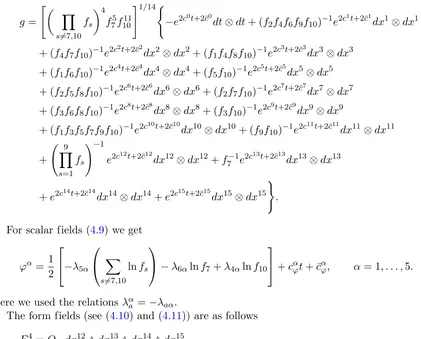
Now we present a cosmologicalS-brane solution from Subsection 4.2.1for the configuration of ten branes under consideration. In what follows the relations εs= +1 and hs= 1/2,s∈S,
For scalar fields (4.9) we get
ϕα= 1
The form fields (see (4.10) and (4.11)) are as follows
where (Ass′) is the Cartan matrix for the KM algebraE10(with the Dynkin diagram from Fig. 1)
and the energy integration constant
ET =
The brane constraints (3.38) are in our case
U1(c) =c3+c4+c10+c12−
Remark 4.2. For a special choice of integration constantsci = 0 andcα
ϕ = 0, we get a solution
governed byE10Toda chain with the energy constraintET = 0. According to the result from [23]
we obtain a never ending asymptotical oscillating behavior of scale factors which is described by the motion of a point-like particle in a billiard B ⊂H9. This billiard has a finite volume since
E10 is hyperbolic.
Special 1-block solution. Now we consider a special 1-block solution (see Subsection4.2.3). This solution is valid when a special set of charges is considered (see (4.16)):
where Q6= 0 and [38]
bs= 2 10
X
s′=1
Ass′ =−60,−122,−186,−252,−320,−390,−462,−306,−152,−230,
s= 1, . . . ,10. Recall that (Ass′) = (Ass′)−1. In this casefs= ( ¯f)bs, where
¯ f(t) =
|Q|p
2/Csinh(√C(t−t0)), C >0, |Q|p
2/|C|sin(p
|C|(t−t0)), C <0,
|Q|√2(t−t0), C = 0
and t0 is a constant.
From (4.17) we get
ET =−620C,
where relation P10
s=1bs =−2480 was used.
For the special solution under consideration the electric monomials in (4.18) have a simpler form
Fs=Qsf¯−2dt∧τ(Is),
where s= 1,2, . . . ,9.
Solution with one harmonic function. LetC = 0 and allci = ¯ci = 0, cαϕ = ¯cαϕ = 0. In this case H = ¯f(t) =|Q|√2(t−t0) >0 is a harmonic function on the 1-dimensional manifold
((t0,+∞),−dt⊗dt) and our solution coincides with the 1-block solution (3.6)–(3.10) (if signνs= −signQs for all s).
Example 4.2. S-brane solution governed by HA(1)2 Toda chain. Now we consider the B11-model in 11-dimensional pseudo-Euclidean space of signature (−,+,. . . ,+) with 4-formF4.
Here we deal with four electric branes (SM2-branes)s1, s2, s3, s4 corresponding to the
4-form F4. The brane sets are the following ones: I
1 = {1,2,3}, I2 = {4,5,6}, I3 = {7,8,9},
I4 ={1,4,10}.
It may be verified that these sets obey the intersection rules corresponding to the hyperbolic KM algebra HA(1)2 with the following Cartan matrix
A=
2 −1 −1 0
−1 2 −1 0
−1 −1 2 −1
0 0 −1 2
(4.19)
(see (3.14) withIsi =Ii).
Now we give a cosmological S-brane solution from Subsection 4.2.1for the configuration of four branes under consideration. In what follows the relationsεs= +1 andhs= 1/2,s∈S, are
used.
The metric (4.8) reads:
g= (f1f2f3f4)1/3
−e2c0t+2¯c0dt⊗dt+ (f1f4)−1e2c
1t+2¯c1
dx1⊗dx1+f1−1e2c2t+2¯c2dx2⊗dx2
+f1−1e2c3t+2¯c3dx3⊗dx3+ (f2f4)−1e2c
4t+2¯c4
+f2−1e2c6t+2¯c6dx6⊗dx6+f3−1e2c7t+2¯c7dx7⊗dx7+f3−1e2c8t+2¯c8dx8⊗dx8
+f3−1e2c9t+2¯c9dx9⊗dx9+f4−1e2c10t+2¯c10dx10⊗dx10
.
The form field (see (4.10)) is as follows
F4 =Q1f1−2f2f3dt∧dx1∧dx2∧dx3+Q2f1f2−2f3dt∧dx4∧dx5∧dx6
The brane constraints (3.38) read in this case as follows
U1(c) =c1+c2+c3 = 0, U1(¯c) = 0,
U2(c) =c4+c5+c6 = 0, U2(¯c) = 0, U3(c) =c7+c8+c9 = 0, U3(¯c) = 0,
U4(c) =c1+c4+c10= 0, U4(¯c) = 0.
SinceF4∧F4= 0 this solution also obeys equations of motion of 11-dimensional supergravity. Special 1-block solution. Now we consider a special 1-block solution (see subsection 4.2.3). This solution is valid when a special set of charges is considered (see (4.16)):
Q2s =Q2|bs|,
For the energy integration constant we have
ET =−11C,
Example 4.3. S-brane solution governed by P10 Toda chain with ET = 0. Now we
consider the B11-model in 11-dimensional pseudo-Euclidean space of signature (−,+, . . . ,+)
with 4-form F4.
These sets obey the intersection rules corresponding to the Lorentzian KM algebra P10 (we
call it Petersen algebra) with the following Cartan matrix
A=
The Dynkin diagram for this Cartan matrix could be represented by the Petersen graph (“a star inside a pentagon”). P10 is the Lorentzian KM algebra. It is a subalgebra ofE10[96,6].
Let us present anS-brane solution for the configuration of 10 electric branes under consid-eration. The metric (4.8) reads:
g=
The form field (see (4.10)) is the following
F4 =Q1f1−2f2f5f10dt∧dx1∧dx4∧dx7+Q2f1f2−2f3f9dt∧dx8∧dx9∧dx10
where (Ass′) is the Cartan matrix (4.20) for the KM algebra P10 and the energy constraint
is obeyed. Here we used the fact that the two sets of linear equations Us(c) = 0, Us(¯c) = 0, s= 1, . . . ,10, have trivial solutions: c= 0, ¯c= 0, due to the linear independence of vectorsUs.
SinceF4∧F4= 0, this solution also obeys the equations of motion of 11-dimensional super-gravity.
Remark 4.3. As pointed out in [96] we do not obtain a never ending asymptotic oscillating behavior of the scale factors in this case since the Lorentzian KM algebraP10 is not hyperbolic
and the corresponding billiard B ⊂H9 has an infinite volume.
Special 1-block solution. Now we consider a special 1-block solution. The calculations give us the following relations
bs= 2 10
X
s′=1
Ass′ =−2, s= 1, . . . ,10,
and hence the special solution is valid (see (4.16)), when all charges are equal
Q2s =Q2,
where Q6= 0. In this case allfs= ¯f−2, where
¯
f(t) =|Q|(t−t0),
and t0 is constant. The metric (4.3) may be rewritten using the synchronous time variablets:
g=−dts⊗dts+At2/7s 10
X
i=1
dxi⊗dxi,
where A > 0 and ts > 0. This metric coincides with the power-law, inflationary solution in
the model with a one-component perfect fluid when the following equation of state is adopted: p= 25ρ, wherep is pressure andρ is the density of fluid [97,98].
5
Black brane solutions
In this section we consider the spherically symmetric case of the metric (4.13), i.e. we putw= 1, M1 =Sd1,g1 =dΩ2d1, where dΩ
2
d1 is the canonical metric on a unit sphere S
d1,d
1 ≥2. In this
case ξ1=d1−1. We put M2 =R,g2=−dt⊗dt, i.e.M2 is a time manifold.
Let C1 ≥ 0. We consider solutions defined on some interval [u0,+∞) with a horizon at
u= +∞.
When the matrix (hαβ) is positive definite and
2∈Is, ∀s∈S,
i.e. all branes have a common time direction t, the horizon condition singles out the unique solution withC1 >0 and linear asymptotics at infinity
qs=−βsu+ ¯βs+o(1),
u→+∞, whereβs,β¯s are constants,s∈S [42,43].
In this case
cA/¯µ=−δ2A+h1U1A+
X
s∈S
hsbsUsA, βs/µ¯= 2
X
s′∈S
wheres∈S,A= (i, α), ¯µ=√C1, the matrix (Ass
′
) is inverse of the generalized Cartan matrix (Ass′) and h1 = (U1, U1)−1 =d1/(1−d1).
Let us introduce a new radial variableR=R(u) through the relations
exp(−2¯µu) = 1− 2µ
Rd¯, µ= ¯µ/d >¯ 0,
where u > 0, Rd¯> 2µ, ¯d =d1−1. We put ¯cA = 0 and qs(0) = 0, A = (i, α), s ∈ S. These
relations guarantee the asymptotic flatness (for R → +∞) of the (2 +d1)-dimensional section
of the metric.
Let us denoteHs=fse−β
su
,s∈S. Then, solutions (4.13)–(4.15) may be written as follows [41,42,43] FunctionsHs>0 obey the equations
d
There exist solutions to equations (5.6)–(5.7) of polynomial type. The simplest example occurs in orthogonal case [58, 47] (for di = 1 see also [56, 57]): (Us, Us′) = 0, for s 6= s′,
(For earlier supergravity solutions see [99,100] and references therein).
In [84, 86, 101] this solution was generalized to a block-orthogonal case (3.3), (3.4). In this case (5.9) is modified as follows
wherebsare defined in (5.1) and parametersPscoincide inside blocks, i.e.Ps=Ps′ fors, s′∈Si, i= 1, . . . , k. The parametersPs6= 0 satisfy the relations [86,101,46]
Ps(Ps+ 2µ) =−B¯s/bs, s∈S, (5.11)
and the parameters ¯Bs/bs coincide inside blocks, i.e. ¯Bs/bs= ¯Bs′/bs′ fors, s′∈Si,i= 1, . . . , k. Finite-dimensional Lie algebras. Let (Ass′) be a Cartan matrix for a finite-dimensional semisimple Lie algebra G. In this case all powers bs defined in (5.1) are natural numbers which
coincide with the components of twice the dual Weyl vector in the basis of simple co-roots [4] and hence, all functionsHs are polynomials, s∈S.
Conjecture 5.1. Let (Ass′) be a Cartan matrix for a semisimple finite-dimensional Lie
algeb-ra G. Then the solutions to equations (5.6)–(5.8) (if exist) have a polynomial structure:
Hs(z) = 1 + ns
X
k=1
Ps(k)zk,
where Ps(k) are constants,k= 1, . . . , ns; ns=bs = 2Ps′∈SAss ′
∈N and P(ns)
s 6= 0,s∈S.
In the extremal case (µ = +0) an analogue of this conjecture was suggested previously in [76]. Conjecture 5.1 was verified for the Am and Cm+1 Lie algebras in [42, 43]. Explicit
expressions for polynomials corresponding to Lie algebras C2 and A3 were obtained in [102]
and [103] respectively.
Hyperbolic KM algebras. Let (Ass′) be a Cartan matrix for an infinite-dimensional
hyperbolic KM algebra G. In this case all powers in (5.1) are negative numbers and hence, we have no chance to get a polynomial structure for Hs. Here we are led to an open problem of
seeking solutions to the set of “master” equations (5.6) with boundary conditions (5.7) and (5.8). These solutions define special solutions to Toda-chain equations corresponding to the hyperbolic KM algebra G.
Example 5.1. Black hole solutions for A1⊕A1, A2 and H2(q, q) KM algebras. Let
us consider the 4-dimensional model governed by the action
S = Z
M
d4zp|g|
R[g]−εgM N∂Mϕ∂Nϕ−
1 2e
2λϕ(F1)2−1
2e
−2λϕ(F2)2
.
Here F1 and F2 are 2-forms, ϕis scalar field andε=±1.
We consider a black brane solution defined on R∗×S2×R with two electric branes s1 and
s2 corresponding to forms F1 and F2, respectively, with the sets I1 = I2 = {2}. Here R∗ is
subset of R, M1 = S2, g1 =dΩ2
2, is the canonical metric on S2, M2 = R, g2 = −dt⊗dt and
ε1 =ε2 =−1.
The scalar products ofU-vectors are (we identifyUi =Usi):
(U1, U1) = (U2, U2) = 1 2+ελ
2 6= 0, (U1, U2) = 1
2−ελ
2.
The matrixA from (3.11) is a generalized non-degenerate Cartan matrix if and only if
2(U1, U2) (U2, U2) =−q,
or, equivalently,
where q= 0,1,3,4, . . .. This takes place when
ε= +1, q= 0,1, ε=−1, q = 3,4,5, . . .
and
λ2= 2 +q 2|2−q|.
The first branch (ε = +1) corresponds to finite dimensional Lie algebrasA1⊕A1 (q = 0),
A2 (q = 1) and the second one (ε = −1) corresponds to hyperbolic KM algebras H2(q, q),
q = 3,4, . . .. In the hyperbolic case the scalar fieldϕis a phantom (ghost). The black brane solution reads (see (5.2)–(5.4))
g= (H1H2)h The moduli functionsHs>0 obey the equations (see (5.6))
d boundary conditions imposed were given in [41, 42, 43]. They are polynomials of degrees 1 and 2 for q= 0 and q = 1, respectively. Forq= 3,4, . . . the exact solutions to equations (5.15) are not known yet.
Special solution with Q21 =Q22. Now we consider the special one-block solution with the functions Hs obeying (5.10) and (5.11). Since bs = 2/(2−q) and ¯Bs = 2Q2s/(q−2) it takes
In this special case the solution (5.12)–(5.14) has the following form:
g=H2
Remarkably, this special solution does not depend uponq. The metric (5.16) coincides with the metric of the Reissner–Nordstr¨om solution (when the Maxwell 2-form is F =√2Q(HR)−2dt∧
In the extremal caseµ→+0 we are lead to the special case of a Majumdar–Papapetrou type solution
g=H2gˆ0−H−2dt⊗dt, ϕ= 0,
Fs=νsdH−1∧dt,
where g0 =P3
i=1dxi⊗dxi,H is a harmonic function on M0 =R3 and νs2 = 1,s= 1,2. Here
νs =−Qs/Q.
6
Conclusions
Here we reviewed several families of exact solutions in multidimensional gravity with a set of scalar fields and fields of forms related to non-singular (e.g. hyperbolic) KM algebras.
The solutions describe composite electromagnetic branes defined on warped products of Ricci-flat, or sometimes Einstein, spaces of arbitrary dimensions and signatures. The metrics are block-diagonal and all scale factors, scalar fields and fields of forms depend on points of some manifold M0. The solutions include those depending upon harmonic functions, S-branes and
spherically-symmetric solutions (e.g. black-branes). Our approach is based on the sigma-model representation obtained in [48] under the rather general assumption on intersections of composite branes (when stress-energy tensor has a diagonal structure).
We were dealing with rather general intersection rules [47] governed by invertible generalized Cartan matrix corresponding to the certain generalized KM Lie algebraG. ForG=A1⊕· · ·⊕A1
(r terms) we get the well-known standard (e.g. supersymmetry preserving) intersection rules [53,54,55,48].
We have also considered a class of special “block-orthogonal” solutions corresponding to semisimple KM algebras and governed by several harmonic functions. Certain examples of 1-block solutions (e.g. corresponding to KM algebras H2(q, q),AE3) were considered.
In the one-block case a generalization of the solutions to those governed by several functions of one harmonic function H and obeying Toda-type equations was presented.
For finite-dimensional (semi-simple) Lie algebras we are led to integrable Lagrange systems while the Toda chains corresponding to infinite-dimensional (non-singular) KM algebras are not well studied yet. Some examples ofS-brane solutions corresponding to Lorentzian KM algebras HA(1)2 =A++2 ,E10 and P10 were presented.
We have also considered general classes of cosmological-type solutions (e.g. S-brane and spherically symmetric solutions) governed by Toda-type equations, containing black brane con-figurations as a special case. The “master” equations for moduli functions have polynomial solutions in the finite-dimensional case (according to our conjecture [41, 42, 43]), while in the infinite-dimensional case we have only a special family of the so-called block-orthogonal solutions corresponding to semi-simple non-singular KM algebras. Examples of 4-dimensional dilatonic black hole solutions corresponding to KM algebrasA1⊕A1,A2 andH2(q, q) (q >2) were given.
We note that the problem of integrability of Toda chain equations corresponding to (non-singular) KM algebras arises also in the context of fluxbrane solutions [44] that have also a poly-nomial structure of moduli functions for finite-dimensional Lie algebras (see also [104]). (For similar S-brane solutions governed by polynomial functions and its applications in connection with cosmological problems see [105,106,107].)
found in [108, 109] and generalized in [110, 111] for arbitrary (anti-)self-dual parallel charge density form of dimension 2m defined on Ricci-flat Riemannian sub-manifold of dimension 4m. In these examples the restrictions on brane intersections (2.11) and (2.12) were replaced by more general condition on the stress-energy tensor: TNM = 0,M 6=N.
It should be noted here that the solutions related to Lorentzian (e.g. hyperbolic) KM algebras considered in Examples4.1–5.1are the new ones. (In Example4.3the brane configuration from [96,6]) was used.)
Acknowledgements
This work was supported in part by the Russian Foundation for Basic Research grant Nr. 07–02– 13624–ofits. We are grateful to D. Singleton for reading the manuscript and valuable comments.
We are also indebted to anonymous referees whose comments have led to the improvement of the paper.
References
[1] Kac V.G., Simple irreducible graded Lie algebras of finite growth, Izv. Akad. Nauk SSSR Ser. Mat. 32
(1968), 1323–1367.
[2] Moody R.V., A new class of Lie algebras,J. Algebra10(1968), 211–230.
[3] Kac V.G., Infinite-dimensional Lie algebras, 3rd ed., Cambridge University Press, Cambridge, 1990.
[4] Fuchs J., Schweigert C., Symmetries, Lie algebras and representations. A graduate course for physicists,
Cambridge Monographs on Mathematical Physics, Cambridge University Press, Cambridge, 1997.
[5] Nikulin V.V., On the classification of hyperbolic root systems of rank three,Proc. Steklov Inst. Math.230
(2000), no. 3, 1–241,alg-geom/9711032,alg-geom/9712033,math.AG/9905150.
[6] Henneaux M., Persson D., Spindel P., Spacelike singularities and hidden symmetries of gravity,Living Rev. Relativity11(2008), lrr-2008-1, 232 pages,arXiv:0710.1818.
[7] Green M.B., Schwarz J.H., Witten E., Superstring theory, Cambridge University Press, Cambridge, 1987.
[8] Saclioglu C., Dynkin diagram for hyperbolic Kac–Moody algebras,J. Phys. A: Math. Gen.22(18) (1989),
3753–3769.
[9] de Buyl S., Schomblond C., Hyperbolic Kac–Moody algebras and Einstein biliards,J. Math. Phys.45(2004),
4464–4492,hep-th/0403285.
[10] Feingold A., Frenkel I.B., A hyperbolic Kac–Moody Algebra and the theory of Siegel modular forms of genus 2,Math. Ann.263(1983), 87–144.
[11] Julia B., Kac–Moody symmetry of gravitation and supergravity theories, in Applications of Group Theory in Physics and Mathematical Physics (Chicago, 1982),Lectures in Appl. Math., Vol. 21, Amer. Math. Soc., Providence, RI, 1985, 355–373.
[12] Mizoguchi S., E10 symmetry in one-dimensional supergravity, Nuclear Phys. B 528 (1998), 238–264, hep-th/9703160.
[13] Nicolai H., A hyperbolic Lie algebra from supergravity,Phys. Lett. B276(1992), 333–340.
[14] Moore G., String duality, automorphic forms, and generalized Kac–Moody algebras, in String Theory, Gauge Theory and Quantum Gravity (Trieste, 1997).Nuclear Phys. Proc. Suppl. 67(1998), 56–67,hep-th/9710198.
[15] Damour T., Henneaux M.,E10,BE10and arithmetical chaos in superstring cosmology,Phys. Rev. Lett. 86 (2001), 4749–4752,hep-th/0012172.
[16] Belinskii V.A., Lifshitz E.M., Khalatnikov I.M., Oscillating regime of approaching to peculiar point in relyativistic cosmology,Usp. Fiz. Nauk102(1970), 463–500 (in Russian).
Belinskii V.A., Lifshitz E.M., Khalatnikov I.M., A general solution of the Einstein equations with a time singularity,Adv. Phys.31(1982), 639–667.
[17] Damour T., Henneaux M., Chaos in superstring cosmology, Phys. Rev. Lett. 85 (2000), 920–923,
hep-th/0003139.
[19] Chitre D.M., Investigations of vanishing of a horizon for Bianchy type IX (the Mixmaster) universe, Ph.D. Thesis, University of Maryland, 1972.
[20] Ivashchuk V.D., Kirillov A.A., Melnikov V.N., On stochastic properties of multidimensional cosmological models near the singular point,Izv. Vyssh. Uchebn. Zaved. Fiz.37(1994), no. 11, 107–111 (English transl.: Russian Phys. J.37(1994), 1102–1106).
[21] Ivashchuk V.D., Kirillov A.A., Melnikov V.N., On stochastic behaviour of multidimensional cosmological models near the singularity, Pis’ma ZhETF 60 (1994), no. 4, 225–229 (English transl.: JETP Lett. 60
(1994), 235–239).
[22] Ivashchuk V.D., Melnikov V.N., Billiard representation for multidimensional cosmology with multicompo-nent perfect fluid near the singularity,Classical Quantum Gravity12(1995), 809–826,gr-qc/9407028.
[23] Ivashchuk V.D., Melnikov V.N., Billiard representation for pseudo-Euclidean Toda-like systems of cosmo-logical origin,Regul. Chaotic Dyn.1(1996), no. 2, 23–35.
[24] Ivashchuk V.D., Melnikov V.N., Billiard representation for multidimensional cosmology with intersecting
p-branes near the singularity,J. Math. Phys.41(2000), 6341–6363,hep-th/9904077.
[25] Damour T., Henneaux M., Nicolai H., Cosmological billiards,Classical Quantum Gravity20(2003), R145–
R200,hep-th/0212256.
[26] Ivashchuk V.D., Melnikov V.N., On billiard approach in multidimensional cosmological models, Gravit. Cosmol.15(2009), 49–58,arXiv:0811.2786.
[27] Cremmer E., Julia B., Scherk J., Supergravity theory in eleven-dimensions,Phys. Lett. B76(1978), 409–412.
[28] Hull C.M., Townsend P.K., Unity of superstring dualities, Nuclear Phys. B 438 (1995), 109–137,
hep-th/9410167.
[29] Witten E., String theory dynamics in various dimensions, Nuclear Phys. B 443 (1995), 85–126,
hep-th/9503124.
[30] Damour T., Henneaux M., Nicolai H.,E10and a small tension expansion of M-theory,Phys. Rev. Lett.89 (2002), 221601, 4 pages,hep-th/0207267.
[31] Gaberdiel M.R., Olive D.I., West P.C., A class of Lorentzian Kac–Moody algebras, Nuclear Phys. B 645
(2002), 403–437,hep-th/0205068.
[32] West P.,E11 and M theory,Classical Quantum Gravity18(2001), 4443–4460,hep-th/0104081.
[33] Schnakenburg I., West P., Kac–Moody symmetries of IIB supergravity,Phys. Lett. B517(2001), 421–428,
hep-th/0107181.
[34] Lambert N.D., West P.C., Coset symmetries in dimensionally reduced bosonic string theory,Nuclear Phys. B615(2001), 117–132,hep-th/0107209.
[35] Englert F., Houart L., Taormina A., West P., The symmetry of M-theories, J. High Energy Phys. 0309
(2003), no. 9, 020, 39 pages,hep-th/0304206.
[36] Englert F., Houart L., West P., Intersection rules, dynamics and symmetries, J. High Energy Phys.2003
(2003), no. 8, 025, 26 pages,hep-th/0307024.
[37] Ivashchuk V.D., Melnikov V.N., Majumdar–Papapetrou-type solutions in sigma-model and intersectingp -branes,Classical Quantum Gravity16(1999), 849–869,hep-th/9802121.
[38] Grebeniuk M.A., Ivashchuk V.D., Sigma-model solutions and intersectingp-branes related to Lie algebras,
Phys. Lett. B442(1998), 125–135,hep-th/9805113.
[39] Ivashchuk V.D., Kim S.-W., Melnikov V.N., Hyperbolic Kac–Moody algebra from intersecting p-branes,
J. Math. Phys.40(1998), 4072–4083,Erratum,J. Math. Phys.42(2001), 5493,hep-th/9803006.
[40] Ivashchuk V.D., Kim S.-W., Solutions with intersectingp-branes related to Toda chains,J. Math. Phys.41
(2000), 444–460,hep-th/9907019.
[41] Ivashchuk V.D., Melnikov V.N., p-brane black holes for general intersections, Gravit. Cosmol. 5 (1999),
313–318,gr-qc/0002085.
[42] Ivashchuk V.D., Melnikov V.N., Black holep-brane solutions for general intersection rules,Gravit. Cosmol. 6(2000), 27–40,hep-th/9910041.
[43] Ivashchuk V.D., Melnikov V.N., Todap-brane black holes and polynomials related to Lie algebras,Classical Quantum Gravity17(2000), 2073–2092,math-ph/0002048.
[44] Ivashchuk V.D., Composite fluxbranes with general intersections, Classical Quantum Gravity19 (2002),