The second term of the asymptotics of the monodromy
map in case of two even edges of Newton diagram
N.Medvedeva, E.Batcheva
Chelyabinsk State University, [email protected]
Abstract
The second term of the asymptotics of the monodromy map of monodromic singular point for some class of vector fields, Newton diagram of which consists of two even edges is computed; in that case the principal term of the asymptotics is an identity mapping. The obtained result allows to formulate the sufficient condition of focus for the singular point from the class under consideration.
AMS subject classification: 34C05, 34C20, 34C35, 58F21
Key words and phrazes: monodromic singular point, center, focus, monodromy map, resolution of singularity, Newton diagram 1
Introduction.
In this paper we calculate the second term of the asymptotics of the monodromy map of monodromic singular point in case when the principal term of the asymptotics is an identity mapping.
It is known ([1],[2]), that the monodromy map (return map) of the monodromic sin-gular point of the analytic vector field on the plane has a linear principal term of the asymptotics
∆(ρ) =Cρ+o(ρ).
The logarithm of the coefficient of this principal term is computed in ([3]) for a so called Γ-nondegenerate vector field. It is expressed via the Taylor coefficients of the principal part of the vector field defined by Newton diagram Γ. If ∆(ρ)≡ρ, then the the singular point is a center. The inequality lnC 6= 0 is the suffucient condition for the singular point to be a focus.
It was found ([3]) if all the edges of the Newton diagram Γ are even, then lnC is identically equal to zero in the class of all the Γ -nondegenerate vector fields having a
1Partially supported by grants d99-411 ISSEP, 9901-00821 and 0001-00745 RFBR.
monodromic singular point. That is impossible to obtain the sufficient condition of focus with help of the principal term of asymptotics.
In this work we consider Γ-nondegenerate vector fields with a monodromic singular point Newton diagram of which consists of two even edges. Under some additional con-ditions we calculate the second term of asymptotics of the monodromy map.
Let us recall some notions connected with the Newton diagram.
We write an analytic vector field (germ) in the neighbourhood of a singular point (x, y) = (0,0) in the form
X(x, y) y
∂ ∂x +
Y(x, y) x
∂
∂y. (0.1)
Here the functions X and Y are divisible by y and x respectively. The vector field (0.1) defines a dynamical system that it will be convenient to write in the form
yx˙ =X(x, y), xy˙ =Y(x, y). (0.2)
Definitions 1. Let
(X
aijxiyj,
X
bijxiyj)
be a Taylor expansion of the right hand-side of the system (0.2). The support of the vector field (0.1) and of the system (0.2) is the set {(i, j) : (aij, bij) 6= (0,0)}. The pair
(aij, bij) is called the vector coefficientof the point (i, j) of the support. The index of the
point (i, j) of the support is the quantity
bij
aij, if aij 6= 0
∞, if aij = 0.
The vector coefficient of any other integer-valued point we define as (0,0). 2. Consider the set
[
(i,j)
{(i, j) +R+2},
whereR2+ is the positive quadrant, the points (i, j) belong to the support. The boundary of the convex hull of this set consists of two open rays and one broken line, which can consist of one point. This broken line is called the Newton diagram of the vector field (0.1). The links of this broken line are called the edges of a Newton diagram, and their end-points are called the vertices of a Newton diagram.
3. Theindex of an edge of a Newton Diagram is the rational number that is equal to the tangent of the angle between the negative direction of the j− axes, and the edge.
Consider the edge of the Newton diagram of the system (0.2) with index α= m
n, where m
n is irreducible fraction. We can group the terms of the Taylor series of the system (0.2)
so that
yx˙ =
∞ P
d=0Xd(x, y), xy˙ = ∞ P
where
Xd(x, y) =
X
ni+mj=d+d0
aijxiyj, Yd(x, y) =
X
ni+mj=d+d0
bijxiyj (0.4)
are quasihomogeneous polynomials of degreed+d0 with weightsnand min the variables x and y respectively, d0 ∈N.
We set Fd(x, y) =Yd(x, y)−αXd(x, y).
Proposition 0.1 ([3]) Let mn be an irreducible fraction. For any quasihomogeneous poly-nomial with weights n and m in the variables x and y respectively the decomposition
R(x, y) =Axs1ys2Y(yn−b
ixm)ki
holds, where bi are distinct nonzero complex numbers and ki ≥0.
Definition. A factor of the form yn−bixm, bi 6= 0, is called the prime factor of the
polynomial R(x, y), the number ki is called themultiplicity of this prime factor.
Definition. A vector field (germ) with Newton diagram Γ is Γ-nondegenerate, if 1) none of the polynomials F0(x, y) corresponding to edges of the Newton diagram Γ has a prime factor of multiplicity larger than one; 2) the index of any vertex not lying on a coordinate axis is different from the indices of the edges adjacent to it.
The set of Γ-nondegenerate vector fields having zero as a monodromic singular point will be denoted by MΓ.
Definition. We call the Newton diagram Γ monodromic, if the set MΓ is nonempty. A Newton diagram is monodromic, if and only if it has one vertex on each coordinate axis and the lengths of the projections of the edges on the coordinate axes are all even numbers ([3]).
Definition. Let α= m
n be an irreducible fraction. The edge of the Newton diagram
with index α will be called even, if one of the numbers m and n and odd otherwise.
Theorem 1 ([3]) Let Γ be a monodromic Newton diagram. ln c= 0 is identically zero on MΓ if and only if all the edges of the Newton diagram Γ are even.
Let the Newton diagram of the vector field V consist of two edges with indices α =
m
n, α˜ =
˜
m
˜
n, where ˜α > α. For each edge we can consider the expansion (0.3) - (0.4).
The polynomials analogous to Xd, Yd, Fd for the edge with index ˜α we denote ˜Xd,Y˜d,F˜d
respectively.
In this paper we prove the following theorem.
Theorem 2 Let Γ be a monodromic Newton diagram consisting of two even edges with indices α = mn and α˜ = mn˜˜ ( ˜α > α) and V be a Γ-nondegenerate vector field having
1)λ = n˜(B0−αA˜ 0)
B0−αA0 >1; λ is irrational number; 2) A0
(B0−αA˜ 0) <0.
Then the monodromy map associated to the origin (taking the axis of abscissa as transversal with a suitable chosen parameter) has possibly after a time reversal the form
∆(ρ) =ρ(1 +F2ρ
1
n +o(ρ
1
n)), ρ→0,
where in case n >1 F2 = 0,
in case n = 1, m˜ – even number, r= ˜mn−˜nm >1,
F2 = 2 +∞ Z
−∞
˜
Φ1(1, ξ)e
ξ
R
0
˜ Φ0(1,τ)dτ
dξ
˜
Φ0(x, y) = ˜ X0(x, y) ˜
nyF˜0(x, y)
, Φ˜1(x, y) = ˜
Y0(x, y) ˜X1(x, y)−Y˜1(x, y) ˜X0(x, y) ˜
nyF˜2 0(x, y)
.
If F2 6= 0,then the origin is a focus.
1
Resolution of the singularity.
Let the Newton diagram of the vector field V consist of two edges with indices α =
m n, α˜ =
˜
m
˜
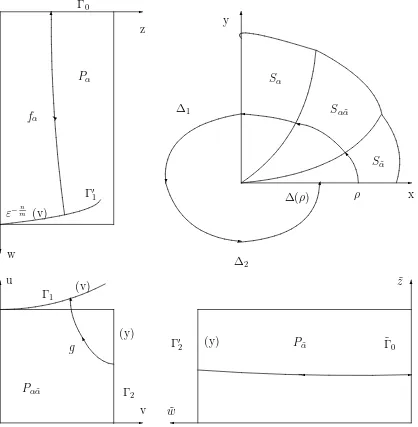
n,where ˜α > α.In according to [3] in such a case the resolution of the singularity
connected with a Newton diagram consists of the following: the first quadrant of the plain (x, y) is broken up into sectors Sα, Sα˜ and Sαα˜, corresponding to the edges and the vertex between them of the Newton diagram.
Let ε >0, δ >0 be small enough. The change of coordinates
x=wzn, y =zm. (1.5) turns the sector Sα ={εxα ≤y≤δ} into the rectangle
Pα={0≤w≤ε
−1
α,0≤z ≤δm1}.
The change of coordinates
x=un˜nvn, y =unm˜vm, (1.6) turns the sector Sαα˜ ={1εxα˜ ≤y≤εxα} into the rectangle
Pαα˜ ={0≤u≤ε1, 0≤v ≤ε2}, where ε1 =ε
1
n˜n( ˜α−α), ε
2=ε
1
n( ˜α−α).
Finally the change of coordinates
x= ˜zn˜, y = ˜zm˜w,˜ (1.7) turns the sector Sα˜ ={0≤y≤ 1εxα˜} into the rectangle
Pα˜ ={0≤w˜ ≤ 1
ǫ, 0≤z˜≤δ
1 ˜
n}.
✲ ✻
❄
✲
✛
✻ ✲ ✻
❑ ❖ ✻
✲ ✛
⑥
♦ ②
✛
❄
✲
✗
x y
ρ ∆(ρ)
Sα
Sαα˜
Sα˜ z
w
Γ0
fα
Pα
Γ′ 1 ε−n
m (v)
Γ1
(v)
g
Pαα˜ Γ2
(y)
(y) Γ′
2 Pα˜ Γ˜0
v w˜
˜ z u
∆1
∆2
Figure 1: Resolution of singularity.
2
Change of coordinates in the sector corresponding
to the edge of a Newton diagram.
Take the change (1.5) in the system (0.2), we obtain
dz
dw =z(Φ0(w,1) +zΦ1(w,1) +...), (2.8) where
Φ0(x, y) =−
Y0(x, y) nxF0(x, y)
Φ1(x, y) =−
m(Y1(x, y)X0(x, y)−X1(x, y)Y0(x, y)) n2xF2
0(x, y)
.
Analogously take the change (1.7), we obtain
d˜z
dw˜ = ˜z( ˜Φ0(1,w) + ˜˜ zΦ˜1(1,w) +˜ ...), (2.9)
where ˜Φ0(x, y),*** ˜Φ1(x, y) are defined at the statement of the theorem 2.
3
Reflected vector fields.
Let Sx and Sy be the reflections of the (x, y)-plane about the x- and y-axes respec-tively, and letSxy =Sx◦Sy. The images of the vector fieldV after reflectionsSx, Sy, Sxy we denote Vx, Vy, Vxy respectively. Consider in the first quadrant four vector fields V, Vx, Vy, Vxy and apply the described resolution of singularity to them. Correspond-ing formulas for the vector field V are given at the previous section. The polinomials analogous to Xd, Yd, Fd,Φd for the reflected vector fields we denote by the same letters
with the corresponding index above. From ([3]) we obtain
Lemma 3.1
Φxd(x, y) = Φd(x,−y), Φ˜xd(x, y) =−Φ˜d(x,−y),
Φyd(x, y) = −Φd(−x, y), Φ˜yd(x, y) = ˜Φd(−x, y),
Φxyd (x, y) = −Φd(−x,−y), Φ˜xyd (x, y) = −Φ˜d(−x,−y).
where d = 0,1.
4
Transition map in the rectangle
P
αα˜.
In this section we denoteF(u, v) be any analytic at the point (0,0) function of variables u, v.
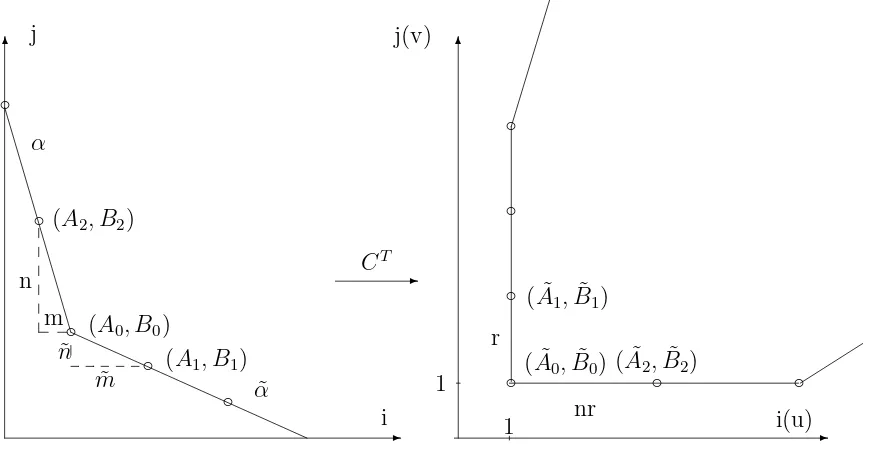
Lemma 4.1 Let (A0, B0) be the vector coefficient of the vertex of the Newton diagram Γ joining its edges, (A1, B1) be the vector coefficient of the nearest to this vertex integer-valued point on the edge with the index α˜; (A2, B2) be the vector coefficient of the nearest to this vertex integer-valued point on the edge with the index α. The change of variables (1.6) in the sector Sαα˜ followed by division by a power function converts fector field V into a vector field
˙
u=u( ˜A0+vr( ˜A1+f1(vr)) +unr( ˜A2+f2(unr)) +uvF(u, v)), ˙
v =v( ˜B0+vr( ˜B1+g1(vr)) +unr( ˜A2+g2(unr)) +uvF(u, v)),
where ( ˜Ai,B˜i) = (r1(Bi −αAi);−n˜r(Bi −αA˜ i)), i = 0,1,2, r = ˜mn−nm, f˜ j, gj−
polynomials, fj(0) =gj(0) = 0, j = 1,2.
Proof. The matrix of exponents corresponding to the change (1.6) has the form
C =
In according to ([3]) the support of the new vector field is the image of the support of the vector field V by means of the mapCT; vector coefficients are transformed by means of matrix C−1
The transformation of the support of the vector field V is shown on the fig.2. From the form of the support of the transformed vector field and from the equality
✲
Figure 2: Transformation of the support.
the conclusion of lemma follows.
From conditions of Γ - nondegegeneracy ˜A0 6= 0, ˜B0 6= 0. After division the system (4.10) on the expression in brackets from the second equation we obtain the system
˙
u=u(−λ1 +vr(a+h
where
λ = n(B˜ 0−αA˜ 0) B0 −αA0
, a= A0B1−B0A1 ˜
n(B0−αA˜ 0)2
( ˜α−α), b= A0B2 −B0A2 ˜
n(B0−αA˜ 0)2
( ˜α−α),
h1, h2− polynomials, h1(0) =h2(0) = 0.
Lemma 4.2 The system (4.11) is reduced to the linear normal form
˙
v =v, y˙ =−1
λy
with help of the C∞
-change of variables of the form
u=y(1 +vr(˜a+ ˜h1(vr)) +unr(˜b+ ˜h2(unr)) +uvF(u, v)), (4.12) where a˜=−ar, ˜b = nrbλ, h˜1, ˜h2− polynomials, ˜h1(0) = ˜h2(0) = 0.
Proof. In according to ([4],[5]) there existsC∞
-change of variabels which linearized the system (4.11). We shall look for it in the form (4.12).
From (4.12) and (4.11) we obtain
˙
y=y(−1
λ+ (a+ ˜ar)v
r+ (b−˜bnr
λ )y
nr +. . .).
Setting equal ˙y to −λ1y) we obtain: ˜a=−ar, ˜b = nrbλ.Lemma is proved.
Because the vector field is Γ - nondegenerate and the singular point is monodromic we have λ >0.
On the plain (y, v) we consider the rectangle 0≤y ≤ε1, 0≤v ≤ε2.LetL1 andL2be the sides of the rectangle not lying on the coordinate axes: L1 ={y=ε1}, L2 ={v =ε2}. Letg :L2 →L1 be a transition map along the trajectories of the linear system
˙
y=y, v˙ =−λv. (4.13)
On L1 we consider the parameter v, on L2 - parametery.
Lemma 4.3 v =g(y) =ε2 y
ε1
λ .
Proof. The trajectory of the system (4.13) goes from the point (y, ε2) to the point (ε1, v) during the time
t=
ε1
Z
y
dy y =−
v
Z
ε2
dv λv.
From here lnε1
y =−
1
λ ln v
ε2, v =ε2
y ε1
5
Parametrisation of transversals.
The change (4.12) converts the segments L1 and L2 into the curves Γ1 and Γ2. On Γ1 we consider the parameter v, on Γ2 −y. Then Γ1 and Γ2 accoding to (4.12) have the following form (r >1):
Γ1 : u=ε1(1 +o(ε1))(1 +O(ε1)v+o(v)), v =v, (5.14)
Γ2 :
u=y(1 +o(ε2))(1 +O(ε2)y+o(y)), v =ε2.
(5.15)
From (1.5) and (1.6) we find that the connection between coordinates (z, w) in the rectangle Pα and (u, v) in the rectangle Pαα˜ is the following
w=unn˜(αα−α˜), z =um˜αv. (5.16)
Analogously from (1.6) and (1.7) we obtain that the coordinates (˜z,w) in the rectangle˜ Pα˜ and (u, v) in the rectangle Pαα˜ are connected by following formulas
˜
w=vn(α−α˜)
, z˜=unvnn˜. (5.17)
Substituting (5.14) in (5.16) we obtain that Γ1 in the coordinates (z, w) has the form
Γ′ 1 :
w=ε∗
1(1 +o(v))
z = ˜ε1v(1 +O(ε1)v+o(v)),
(5.18)
where ε∗ 1 =ε
−n
m(1 +o(ε1)), ε˜1 =ε
˜
m α
1 (1 +o(ε1)).
Analogously substituting (5.15) in (5.17) we obtain that Γ2 in coordinates (˜z,w) has˜ the form
Γ′ 2 :
˜ w= 1
ε
˜
z = ˜ε2yn(1 +O(ε2)y+o(y)),
(5.19)
where ˜ε2 =ε
n
˜
n
2(1 +o(ε2)).
6
Transition maps in the rectangels corresponding
to edges.
Consider in coordinates (˜z,w) two transversals ˜˜ Γ0 = {w˜ = 0} with parameter ρ = ˜z and Γ′
2 (see (5.19)) with parameter y. Calculate the coefficients of the transition map fα˜ : Γ
′
2 →Γ˜0.
Lemma 6.1 The map fα˜ has the asymptotics
where
˜ d= ˜ε2e
−
1
ε
R
0
˜ Φ0(1,ξ)dξ
, (6.21)
˜ d1
˜ d =−
1
ε
Z
0 ˜
Φ1(1, ξ)e
ξ
R
0
˜ Φ0(1,τ)dτ
dξ+ O(ε˜2)
d , if n= 1, ˜
d1 =O(ε2) if n > 1. (6.22)
Proof. We look for the solution ˜z( ˜w, ρ) of the equation (2.9) with the initial condition ˜
z(0, ρ) in the form
˜
z( ˜w, ρ) =ρ( ˜C0( ˜w) + ˜C1( ˜w)ρ+...), (6.23)
where ˜C0(0) = 1, C˜i(0) = 0 as i≥0.
Solving corresponding equations in variations we obtain
˜
C0( ˜w) = e
˜
w
R
0
˜ Φ0(1,ξ)dξ
, C˜1( ˜w) = ˜C0( ˜w) ˜
w
Z
0 ˜
C0(ξ) ˜Φ1(1, ξ)dξ. (6.24)
For the map ρ=fα˜(y) from (6.23) and (5.19) we obtain the equation ˜
C0ρ+ ˜C1ρ2+...= ˜ε2yn(1 +O(ε2)y+o(y)), (6.25) where ˜Ci = ˜Ci(1ε), i= 0,1.
We shall look for ρ=fα˜ in the form (6.20). Substituting (6.20) in (6.25) we obtain ˜
C0dy˜ n(1 + ˜d1y+o(y)) + ˜C1d˜2y2n(1 + ˜d1y+o(y))2+o(y2) = ˜ε2yn(1 +O(ε2)y+o(y)). Let n= 1. Then
˜
C0dy(1 + ˜˜ d1y+o(y)) + ˜C1d˜2y2(1 + 2 ˜d1y+o(y)) +o(y2) = ˜ε2y(1 +O(ε2)y+o(y))
or ˜C0dy˜ + ( ˜C0d˜d˜1+ ˜C1d˜2)y2+o(y2) = ˜ε2y+ ˜ε2O(ε2)y2+o(y2)
Setting equal coefficients in the equal powers ofy, we obtain the conclusion of lemma. In the case that n >1 we obtain the same expression for ˜d, and ˜d1 = O(ε2). Lemma is proved.
Consider in coordinates (z, w) two curves: Γ0 = {w = 0} with parameter ρ =z and Γ′
1 (see (5.18)) with parameter v. It is evident, that the transition map fα : Γ′1 →Γ0 has the asymptotics
ρ=dv(1 +d1v+...) (6.26)
As in the proof of Lemma 6.1 we obtain that
d= ˜ε1e −
ε∗
1
R
0
Φ0(ξ,1)dξ
7
Coefficients of the composition of the transition
maps.
The monodromy map ∆ is the composition of the following maps:
∆ = ∆2◦∆1,
where ∆1 is a transition map for the upper half-plane which transforms the positive x-half-axis near the origin into the negative x-half-axis in the positive direction along the trajectories of the vector field, and ∆2 is the analogous map for the lower half-plane (see fig.1).
The maps analogous to fα, fα˜, g for the reflected vector fields we denote by the same letters with corresponding index above. Then
∆1 =fαy˜ ◦(gy)
1 . Observe that all the analogous to g transition maps for the reflected vector fields have the same formula, because the number λ is the same for all of them ([3]).
The maps fα and fα˜ are defined by formulas (6.26) and (6.20) respectively. Inverse maps have respectively forms
v = (fαy)−1
It is easy to compute, that
y=g−1
(v) =ε−λγv
1
λ.
Taking into account that λ >1 we obtain in consecutive order:
Analogously ∆x
cx is a coefficient of the principal term of the asymptotics of the monodromy
map ∆, then in our case of even edges it is equal to 1, hence
We show, that the value d
dy is bounded as ε→0. Really from the formula (6.27) and
Limits in the integral in the exponent are not symmetric, because the quantity
ε∗ 1 =ε
−n
contains o - small, which for the reflected vector field can be differ from the analogous quantity for the initial vector field.
Therefore
where the limits in the integral in the first exponent are symmetric, and both of the ends of the segment I(ε) have the asymptotics (7.32). Because from Γ - nondegeneracy conditions
Φ0(ξ,1) =O( 1
ξk), k ≥1, (7.34)
asξ → ∞, then the integraal in the first exponent turns to the finite limit asε →0. From (7.34) we also obtain, that the integral in the second exponent in the formula (7.33) is O(εmnk)ε
−n
m
1 o(ε1) =o(ε1). Hence the second exponent turns to 1 asε→0. From here the ratio d
dy is bounded. Notice that if m is even the integrand in the first exponent (7.33) is
odd and so
Because the ratio d
dy is bounded we have c1 →0 as ε→0. Analogously cx1 →0 asε →0. From here and because F2 is undependent onε we obtain thatF2 = 0.
Let n= 1.
Because in this casem is even, that from (7.30),(7.28), (7.29), (7.35), (7.36) we obtain that
From here and from lemma 3.1 we obtain, that
From here, from (7.39) and (7.37) we obtain, that
Investigate the asymptotics of the integral in the formula (6.22) for the quantity d˜1
˜
d.
The edge with index ˜α is situated on the line l : ˜ni+ ˜mj= ˜d0, the edge with indexα is situated on the line ni+mj =d0.
Let (i0, j0) be the coordinates of the vertex, joining these edges. Then
ni0+mj0 =d0, ˜ni0+ ˜mj0 = ˜d0.
Consider the right linel1,passing throw the point (i0−m, j0+n) in parallel tol.Then l1 has the equation ˜ni+ ˜mj =dand ˜n(i0−m) + ˜m(j0+n) = d.From here d−d˜0 =r >1. Therefore the supports of the functions ˜X1 and ˜Y1 do not lie on the right line l1, hence they lie lower. Because n = 1, then the upper points of these supports lie not above the horizontal line j =j0. So the powers of the polynomials ˜X1(1, ξ) and ˜Y1(1, ξ) are not greater than the power j0 of polynomials ˜X0, Y˜0, F˜0.Therefore ˜Φ1(1, ξ) =O(ξ1m), m≥1
as ξ→ ∞.
From here and from the formula (7.36) we obtain, that the integrand in (6.22) is O(ξl−1b0). So from the condition b0 < 0 the integral in the formula (6.22) turns to the finite limit as ε→0.
We proved early, that two last terms in (7.40) turn to 0 as ε → 0. From here and because the quantity F2 does not depend on ε we conclude that
F2 = lim
Continue the proof of the theorem. Twice changing the variable on the opposite one we obtain
From here, from (6.22) and (7.41) we obtain
F2 = 2 lim
References
[1] V.I.Arnol’d and Yu.S.Il’yashenko, Ordinary differential equations. 1. in: ”Sovre-mennye problemy matematiki. Fundamental’nye napravleniya, Vol.1, Itogi Nauki i Tekhniki, VINITI AN SSSR, Moscow, 1985, 7-149 (English: Encyclopaedia of Math-ematical Science, Vol.1, Springer, Heidelberg).
[2] N.B.Medvedeva, The principal term of the first return function of a monodromic singular point is linear, Sibirskii matematicheskii zhurnal. 1992, Vol.33, No.2 p.116-124.
[3] F.S.Berezovskaja and N.B.Medvedeva, A complicated Singular point of ”Center-focus” type and the Newton diagram, Selecta Mathematica Vol.13, No 1, 1994, p.1-15.
[4] Yu.S.Il’yashenko, The memoir of Dulak ”About the limit cycles” and the ajacent questions of the local theory of the differential equations, Uspekhi Mat. Nauk 40(1985), p.41-78.