CONDITIONAL RANDOM FIELDS FOR THE
CLASSIFICATION OF LIDAR POINT CLOUDS
J. Niemeyer1, C. M allet2, F. Rottensteiner1, U. Sörgel1 1
Institute of Photogrammetry and GeoInformation , Leibniz Universität Hannover, D-30167 Hannover, Germany - (niemeyer, rottensteiner, soergel)@ipi.uni-hannover.de
2
Université Paris Est, Laboratoire MATIS, Institut Géographique National, F-94165 Saint-Mandé, France - [email protected]
KEY WORDS : Conditional Random Fields, 3D Point Cloud, LiDAR, Classification
ABS TRACT:
In this paper we propose a probabilistic supervised classification algorithm for LiDAR (Light Detection And Ranging) point clouds. Several object classes (i.e. gr ound, building and vegetation) can be separated reliably by considering each point's neighbourhood. Based on Conditional Random Fields (CRF) this contextual information can be incorporated into classification process in order to improve results. Since we want to perform a point-wise classification, no primarily segmentation is needed. Therefore, each 3D point is regarded as a graph's node, whereas edges represent links to the nearest neighbours. Both nodes and edges are associated with features and have effect on the classification. We use some features available from full waveform technology such as amplitude, echo width and number of echoes as well as some extracted geometrical features. The aim of the paper is to describe the CRF model set-up for irregular point clouds, present the features used for classification, and to discuss some results. The resulting overall accuracy is about 94 %.
1. INTRODUCTION
1.1 Motivation
Airborne LiDAR (Light Detection And Ranging) has become a standard technology for the acquisition of elevation data. Especially in urban areas, the classification of a point cloud is an important, but challenging task in order to derive products like 3D city models. Consisting of many different objects such as buildings, ground and vegetation, urban scenes are complex. As a consequence three-dimensional point clouds are difficult to classify.
Common approaches classify each point independently of its neighbourhood. However, incorporating this contextual information can improve the quality of the results significantly. In this work we present a supervised classification method of 3D point clouds based on Conditional Random Fields, which is able to take into account contextual correlations. Several object classes can be distinguished. We do not carry out a segmentation before classification, but we directly classify each point individually .
1.2 Related Work
In urban areas the most important objects are buildings. Consequently, many publications can be found in literature dealing with this topic, e.g. (Rottensteiner & Briese, 2002). The detection of urban vegetation has become increasingly important. M any applications based on city models require more realistic descriptions. For instance, trees and hedges have an important effect on a flooding- or emission simulation. Therefore, accurate information about vegetation is needed. The classification of vegetation can benefit from full waveform LiDAR technology (Wagner et al., 2008). An analysis of the temporal behaviour of the received waveform provides some additional information about the illuminated objects. On the one
hand, we are able to acquire multiple echoes within one waveform, which give hints of the vertical distribution of objects within a footprint. Thus, especially in vegetated areas, the point density gets improved, and the objects are better described in 3D. On the other hand, information concerning the slope and reflectance of illuminated objects can be derived. Usually, Gaussians are fitted into the continuous backscattered waveform in order to detect echoes (Wagner et al., 2006). Object size and radiometric object properties have effect on the echoes’ amplitude. In addition, the echo width can be a good indicator for vegetation (Rutzinger et al., 2008), because it is narrow on ground and gets broadened in tree regions.
Several approaches consider the task of classifying an entire point cloud and assigning the points to different object classes. For this purpose, some investigations have been spent on Support Vector M achines (SVM ), e.g. (M allet, 2010). Although SVM s are able to handle high-dimensional feature spaces, they are restricted to local classification of points or segments, respectively. M ost of the common classifiers solely take into account local features in order to assign a point to one of the classes to be discerned.
However, some improving hints can be integrated into decision process by considering contextual knowledge. Especially in computer vision an approach for image classification has become increasingly popular: Conditional Random Fields (CRF). Lafferty et al. (2001) originally introduced CRFs for labeling one-dimensional sequence data. Since the approach was adapted to the classification of imagery by Kumar and Hebert (2003), CRFs have been applied to various tasks in computer vision. Recently, in remote sensing, some applications dealing with object detection by using CRFs were published. Nevertheless, this works mainly focus on optical images. As learning and inference CRFs are computational expensive, the classification of large LiDAR point clouds is a challenging task. Some initial applications dealing with terrestrial point clouds can be found in the fields of robotics and mobile laser scanning. International Archives of the Photogrammetry, Remote Sensing and Spatial Information Sciences, Volume XXXVIII-4/W19, 2011
For instance, Anguelov et al. (2005) perform a point-wise classification on terrestrial laser scans. Lim and Suter (2009) present an approach which first over-segments a terrestrial point cloud acquired by mobile mapping and then perform a segment-wise classification based on CRFs. One approaches dealing with a CRF applied to airborne LiDAR point cloud is described from Shapovalov et al. (2010). However, they first perform a segmentation on the point cloud and classify the segments in a second step . This aspect helps to cope with noise, but small objects with sub-segment size cannot be detected. A more accurate method would be a point-wise classification. Compared to segment-based labeling this approach requires higher computational costs, but more small objects can be detected correctly .
In this paper we propose a method for a point-based classification to approach of full waveform airborne LiDAR data based on Conditional Random Fields. In Section 2 the
CRFs provide a probabilistic framework for the estimation of random variables that depend on each other, and can be used for classification tasks. In contrast to common classifiers the results can be improved by modelling the influence of the neighbourhood on an object. Context knowledge is generically learned by training, so that a CRF-based approach is more flexible than a model-based method.
Belonging to the group of undirected graphical models, a CRF represents a scene by a graph consisting of nodes S and edges E. Given the observed data x and unknown class labels y, these discriminative models estimate the posterior distribution P(y|x) directly. All nodes are associated to corresponding labels simultaneously. The main equation for CRF is given by
Ai = association potential for node i
Iij = interaction potential of nodes i and j
Z = partition function Ni = neighbourhood of node i
CRF are a generalisation of M arkov Random Fields (M RF), because more contextual knowledge conditioned to the data can be integrated in the interaction of nodes.
2.1 Association Potential
The association potential determines the most likely class label yi of a single node i given the observations x. It is related to the
probability P:
(1)
Theoretically, the result of any classifier can be used. We utilize a generalized linear model (GLM , Eq. 3) here. It depends on the corresponding node feature vector hi(x).
(3)
Parameter vector w contains weights for the features associated to each class l. It is derived in the training step (Section 2.3).
2.2 Interaction Potential
The pairwise potential Iij (Eq. 4) provides a possibility to model
the interaction of contextual relations of neighbouring objects in the classification process. Therefore, for each edge connecting two nodes i and j an edge feature vector µij depending on the data x is generated.
( ) (4)
In our implementation we use generalized linear models again (Eq. 4). Relations of the local neighbourhood can be considered by using the following function:
( ) ( ) (5)
where ( ) {
In Eq. 5, the first term δ compares the two node labels yi and yj.
Different labels are penalized, whereas corresponding labels are preferred. The degree of penalization depends on the edge feature vector µij and weight vector v, which is learned in
training.
2.3 Training and Inference
The weights wlfor node features in association potential (Eq. 3) and v for the edge features in interaction potentials (Eq. 5) can be derived by training. For this purpose, a part of a fully labeled point cloud is required. The training task is a nonlinear numerical optimization problem, in which a cost function (optimization objective) is minimized. This topic has been widely discussed in literature. For instance in (Nocedal & Wright, 2006) several approaches are presented.
∑ ∑ ∑ ∑ ( ) normalizes the potentials to a probability value. Since our graph structure is complex and may have cycles, no explicit computation by message passing algorithms is possible. As a consequence it must be solved approximately. According to Vishwanathan et al. (2006) we use Loopy-Belief-Propagation for message passing and the common quasi-Newton limited memory Broyden-Fletcher-Goldfarb-Shanno (L-BFGS) method for optimization of objective f=-log(P(θ|X,Y)) with θT= ( vT).
3. METHOD
Our approach starts with a pre-processing step based on the original LiDAR point cloud. It computes the input required for the CRF and includes two operations: First, the graphical model is constructed. In particular, each point corresponds to a node and is linked by edges to the points in its spatial vicinity. We International Archives of the Photogrammetry, Remote Sensing and Spatial Information Sciences, Volume XXXVIII-4/W19, 2011
get a list of all nodes and edges. In the second part of the pre-processing step , several features are extracted. In training stage, the parameter weights are learned. Therefore, a labeled training site is necessary. Finally, these learned weights are used for the classification process of an unlabeled scene. The result is a fully labeled point cloud of the test site together with the probabilities of these classes’ assignments. In the following sections the methodology of our classification approach is described in detail.
3.1 Pre-processing
3.1.1 Graph construction: As already mentioned in Section 2, a CRF is a graphical model consisting of nodes S being linked by edges E. This representation is required for message passing algorithms in training and classification stage to estimate the most likely label configuration. Graph construction is only based on the geometrical information given by x, y, z-coordinates of the points.
There is a notable difference to CRFs in field of computer vision. Images are typically aligned in a regular grid. Common methods deal with classification tasks of pixels or pixel-blocks (Kumar & Hebert, 2003), which are still in lattice form. This property enables a simple graph structure, since each pixel (block) has the same number of neighbours, usually four or eight. In contrast to this, a 3D LiDAR point cloud is irregular and has a more complex topology , so the structure of the undirected graph must be different from the type of graph that is generally used for image-based classifications.
Unlike Shapovalov et al. (2010), we want to classify every LiDAR point rather than segments. Thus, each point corresponds to a node in our graph. Accordingly, edges link the points/nodes that are geometrically close to each other. Compared to other approaches, this methodology enables an accurate classification in which small objects described by a few points are preserved, because there is no smoothing in segmentation step and we use the original point cloud. However, computational complexity is a drawback due to the fact that the resulting graph structure may consists of hundreds of thousands of nodes and edges.
For the graph construction, each point is linked to its nearest neighbours within a manual defined distance by edges. Thus, the number of edges per node may vary. In a 3D point cloud it is obvious to search neighbours within a sphere. A very local vicinity would be considered in this case. Nevertheless, our experiments have shown that especially the height differences improve object classification. This is why links to points at other height levels are important, which often belong to another object class. This significant information is not necessarily available with search inside spherical volumes or by k nearest neighbour approach. In our method the neighbouring points are searched within a cylinder of radius 1 m perpendicular to the xy-plane. Thus, more points are linked by edges.
Both nodes and corresponding edges of the graph are represented in list form and get associated with features in order to enable classification. This is described in the next sections.
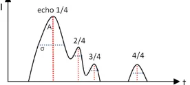
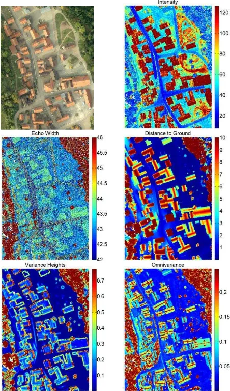
3.1.2 Node Features: The classification of the point cloud is based on LiDAR features only . Since full waveform laser scanners provide additional information, we decided to classify a point cloud acquired by such sensors. Thus, more features per point are available describing the shape of the received signal (e.g. amplitude A and width σ, Fig. 1) and the number of echoes. Especially the classification of vegetation may be improved by these features.
Fig. 1: Backscattered signal recorded by full waveform laser scanner. Gaussians are fitted to the sampled signal. The features amplitude A and width σ can be used to characterise the echoes.
The selection of suitable features is an important field of research. In our previous work (M allet et al., 2008) we presented eight LiDAR features and determined their contribution to classification results. Accordingly, we separate our features into two groups. The first one contains features obtained from full waveform laser scanning. The second group consists of features based on the local point geometry.
Amplitude: The term intensity is not yet defined clearly (Wagner et al., 2008), but the amplitude A of the estimated Gaussian is most commonly referred to as intensity. Thus, this value is related to the reflectivity of the illuminated object. Here, the values were corrected by the approach presented from Höfle and Pfeifer (2007) in order to eliminate the dependency between amplitude and incidence angle of laser beam and object surface.
Echo width: For full waveform laser scanning usually Gaussians are fitted to the waveform to model the echoes. In addition to amplitudes, the widths σ of the Gaussians can be used to describe echoes (Fig. 1). This feature is especially important for detection of vegetation since branches widen the echoes. Advanced object information concerning the type of vegetation can be derived. (M allet et al., 2008)
Normalized echo number: With the new generation of laser scanner sensors, several backscattered echoes of vertically distributed objects in the beam can be recorded now from a single pulse. For each echo we get information about the number of the current echo and the total number of echoes within the waveform.
Difference first-last pulse: This feature describes the geometrical height difference between the first and the last echo of a single emitted pulse. High differences hint primarily at vegetation or at the edges of building roofs. If there is only one echo, the value of this feature is zero.
In addition to the full waveform features some geometric features are extracted for every LiDAR point cloud, too:
Distance to Ground: According to M allet (2010), for each echo the height above ground can be approximated without a need of a Digital Terrain M odel (DTM ) in almost flat areas. Therefore, the height of the lowest 3D-point within a cylinder centred at the current point is used to approximate ground level. International Archives of the Photogrammetry, Remote Sensing and Spatial Information Sciences, Volume XXXVIII-4/W19, 2011
This feature is very important to separate objects like vegetation and building roofs from ground. A flat plane, for instance, might be part of a roof or of the ground. Since the chosen radius of the cylinder is bigger than the largest building in the scene (here 20 m), the points of this plane can be classified correctly.
Variance normals: The variance of normal vectors in a local spherical neighbourhood (radius 1.25 m) will be small for smooth areas like roofs, or ground.
Elevation variance: The variance of the point elevations in the current spherical neighbourhood indicates whether significant height differences exist, which is typical for vegetated areas.
Residuals of planar fit: Points in the local neighbourhood of each current point are used to fit a plane (L2 norm) by a robust M -estimator. Information about roughness can be derived by analysing the residuals. The value will be high in vegetation areas and near zero for points describing ground and roofs.
Omnivariance: Gross et al. (2007) show that the distribution of points in a local neighbourhood (radius 1.25 m) can be an significant feature for point cloud classification. For the point distribution within this neighbourhood a covariance-matrix Σ and its three eigenvalues λ1-3 are computed. This allows us to
distinguish between a linear, a planar or a volumetric distribution of the points. The feature omnivariance is defined as
√∏
(7)
Low values will correspond to planar regions (ground, roofs), and linear structures whereas higher values are expected for areas with a volumetric point distribution like vegetation.
Planarity: Another relevant eigenvalue-based feature is the planarity (λ2-λ3)/λ1, which is high for roofs and ground, but low
for vegetation.
Altogether, we use 10 features for our classification task. They are computed for each 3D point and associated to each node in the CRF by a feature vector hi(x) (Eq. 3) of dimension 10 in this case. Note that the values are not homogeneously scaled due to the different physical interpretation and units of these features. For instance the normalized echo number ranges from 0 to 1, whereas the amplitude has a much higher variance and ranges up to 120. For getting representative parameter weights in CRF-training step, a normalisation to standard normal distributed features is required to align the ranges.
3.1.3Edge Features: Having determined the node features
hi(x) in the way described in the previous section, the edge feature vector µij(x) used for the interaction potential (Eq.5) need to be obtained. We use the difference between the feature vectors of two adjacent nodes I and j for that purpose, thus:
µij(x) = hi(x) - hj(x) (8)
Depending on the current node labels configuration, several combinations are more likely and typical structures can be learned. As a result, the interaction potential causes a smoothing effect.
3.2 Training and Inference
Following Vishwanathan et al. (2006), we utilize the iterative Loopy Belief Propagation (LBP) algorithm, which is a frequently used message passing algorithm for graphs with cycles.
The weight parameters wl and v are determined by training. Therefore, nonlinear optimization is done with the quasi-Newton method L-BFGS (Vishwanathan et al., 2006). The result of inference with an unlabeled point cloud and trained weights is a probability value for each point belonging to each class. M aximum a posteriori estimation (M AP) selects the highest probability and finally labels the point to the corresponding object class.
4. EVALUATION
4.1 Dataset
Our classification framework is validated with a flight strip of a rural scene called Bonnland (see Fig. 3a). The test area consists of scattered buildings with different shapes, streets, grassland, Fig. 2: Sampled feature characteristics in different object classes. Plots show a) aerial image as reference, b) amplitude, c) echo width, d) distance to ground, e) variance of heights and f) omnivariance.
some single trees and forested regions. In 2008, data acquisition was done with a RIEGL LM S-Q560 full-waveform laser scanner. In an area of about 2.02 ha nearly 760,000 points were recorded. This corresponds to a mean echo density of about 3.7 points/m2. The raw data points are delivered with 3D coordinates and the attributes amplitude, echo width, number of echo and total echoes within the waveform. Table 1 depicts the distribution of the echo numbers in the area, whereas Table 2 demonstrates the distribution for the three object classes of interest gr ound, buildings and vegetation in the scene.
# echoes 1 2 3 4 5
Distribution (%) 87.4 11.1 1.4 0.08 <0.01 Table 1: Distribution of multi echoes
reference class # points percentage
ground 432449 56.9 %
building 59728 7.9 %
vegetation 267613 35.2 % Table 2: Distribution of object classes in ground truth.
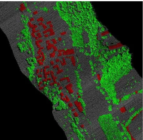
We divided the whole area into three parts, namely Nor th, Middle, and South, which were used to perform cross-validation (red lines in Fig. 3a). The manually labeled point cloud for ground truth is shown in Fig. 3b.
Fig. 3: (a) Aerial image of scene consisting of three parts Nor th, Middle, and South. (b) Ground Truth of LiDAR point cloud (grey = gr ound, red = building, green = vegetation).
4.2 Computational complexity
For this data set we used a radius of 1 m for the search of neighbouring points in the point cloud. Especially the points representing vegetation have a low voluminous density, and the height of the point above ground is an important hint to assign it to the correct object class. We chose a cylinder for vicinity search in order to take care of vertical restrictions due to the topography of objects (Section 3.1.1). This results in a large graphical structure. As can be seen in Table 3, we constructed a separate graph structure for each of the three subsets. Altogether, the 760K points were connected by 4.6 million edges. Since the number of neighbours depends on a radius and is not fixed, it may vary. In the mean a point is linked to six neighbours.
North M iddle South Sum #nodes 321,575 224,669 213,546 759,790 #edges 1,951,603 1,376,441 1,291,278 4,619,322 Table 3: Number of nodes and edges of 3 test parts in Bonnland.
4.3 Results
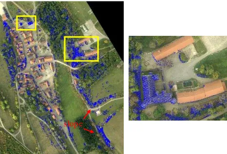
In this study our approach is evaluated by three-fold cross-validation. Parameters are trained on two parts of the data and tested on the third. This is done three times (i.e., folds), each time with another combination of the data subsets. Finally, we report the mean performance parameters of all three subsets. The result is shown in Fig. 4. Altogether, the classification performed well for the three object classes gr ound, building and vegetation. It is expressed by the overall accuracy of 94 % (Table 4). Correctness as well as completeness rates are between 91.2 % and 95.3 %. Only the correctness rate of buildings is a bit lower (87.7 %) due to some misclassifications in the South-East (Fig. 5a, red arrows). Here, terrain slopes are assigned to building instead of gr ound. The reasons are broadened echo widths and high distance-to-ground values, due to the underlying terrain. This topography does not appear in the other two training folds which were used for training, so it could not be learned and leads to misclassifications.
Fig. 4: Result CRF-classification (grey = gr ound, red = building, green = vegetation).
The other main problems are three undetected buildings in the Northern part (yellow boxes Fig. 5a). Their roofs consist of different materials and have completely other reflectivity properties. Those buildings are not contained in the other two subsets which were used for training, so the errors are due to unlearned feature characteristics again. Fig. 5b depicts this issue. All misclassified points are displayed in blue. M any errors appear on the building roof at the left side with strongly reflecting material, while the buildings at the right are classified correctly. Points have similar features to most other buildings here.
Classified
Re
fe
re
nc
e
gr ound building vegetation corr.
gr ound 95.3 1.0 3.7 95.3
building 7.4 87.7 4.9 87.7
vegetation 6.5 0.2 93.3 93.3
compl. 95.0 91.2 93.0 94.0
Table 4: Confusions matrix [%] with completeness (comp.) and correctness (corr.) rates.
Fig. 5: Distribution of classification errors in the entire scene (a) and subset of one misclassified building (b). Incorrect assigned points are displayed in blue. Slope is marked by red arrow, buildings with different features are marked by yellow boxes.
5. CONCLUS ION AND OUTLOOK
Our work introduced a probabilistic method for a point-wise classification approach of a LiDAR point cloud based on Conditional Random Fields (CRF). The assignment to one of the three object classes vegetation, building and gr ound is based on two groups of features: On the one hand, for each 3D point some features can be derived that describe the geometry . On the other hand, new full waveform laser scanning sensors provide additional parameters like amplitude, echo width and number of echoes. The good results yielded in this work demonstrate that Conditional Random Fields seems to be a powerful method for classification of point clouds.
Further investigations will concentrate on a more sophisticated model of the interaction potential to incorporate global context . We live in man-made environments and all the objects are well structured. Therefore, in urban areas, the objects arrangements provide useful hints on the nature of these objects. For instance, buildings and trees are allocated along the streets. This context knowledge can be used to improve point cloud classification. M oreover, we are going to validate the CRF approach with more complex data sets and compare the results with different classifiers.
ACKNOWLEDGEMENTS
We used the "M atlab toolbox for probabilistic undirected models", developed by M ark Schmidt. This software can be found at http://www.cs.ubc.ca/~schmidtm/Software/UGM .html (last access M arch 15, 2011). This work is funded by the German Research Foundation (DFG) among project ID 134144775.
REFERENCES
Anguelov, D , Taskar, B., Chatalbashev, V., Koller, D., Gupta, D., Heitz, G. and Ng, A., 2005. Discriminative learning of markov random fields for segmentation of 3d scan data. In: Pr oc. of the IEEE CVPR 2005, Vol. 2, pp. 169–176.
Gross, H., Jutzi, B. and Thoennessen, U., 2007. Segmentation of tree regions using data of a full-waveform laser. Inter national Ar chives of Photogr ammetr y, Remote Sensing and Spatial Infor mation Sciences, Vol. XXXVI, part 3, pp. 57–62.
Höfle, B. and Pfeifer, N., 2007. Correction of laser scanning intensity data: Data and model-driven approaches. ISPRS Jour nal of Photogr ammetr y and Remote Sensing, Vol. 62, Issue 6, pp. 415–433.
Kumar, S. and Hebert, M ., 2003. Discriminative random fields: A discriminative framework for contextual interaction in classification. In: Pr oc. of IEEE Inter national Confer ence on Computer Vision (ICCV '03), Vol. 2, pp. 1150-1157.
Lafferty, J., M cCallum, A. and Pereira, F., 2001. Conditional random fields: Probabilistic models for segmenting and labeling sequence data. In: Pr oc. of Inter national Confer ence on Machine Lear ning, pp. 282–289.
Lim, E.H. and Suter, D., 2009. 3d terrestrial lidar classifications with super-voxels and multi-scale conditional random fields. Computer -Aided Design, Vol. 41, No. 10, pp. 701–710.
M allet, C., 2010. Analysis of Full-Wavefor m lidar data for ur ban ar ea mapping. PhD thesis, Télécom ParisTech.
M allet, C., Bretar, F. and Soergel, U., 2008. Analysis of full-waveform lidar data for classification of urban areas. PFG, Vol. 5, pp. 337–349.
Nocedal, J. and Wright, S.J., 2006. Numer ical optimization. Springer, 2nd edition, New York, NY, USA.
Rottensteiner, F. and Briese, C., 2002. A new method for building extraction in urban areas from high-resolution LIDAR data. In: Inter national Ar chives of Photogr ammetr y, Remote Sensing and Spatial Infor mation Sciences, Vol. XXXIV, part 3A, pp. 295-301.
Rutzinger, M ., Höfle, B., Hollaus, M . and Pfeifer, N., 2008. Object-based point cloud analysis of full-waveform airborne laser scanning data for urban vegetation classification. Sensor s, Vol. 8, Issue 8, pp. 4505–4528.
Shapovalov, R., Velizhev, A. and Barinova, O., 2010. Non-associative markov networks for 3d point cloud classification. In: Pr oc. of the ISPRS Commission III symposium - PCV 2010, IntAr chPhRS, Vol. XXXVIII, part 3A, Saint-M andé, France, pp. 103–108.
Vishwanathan, S., Schraudolph, N., Schmidt, M . and M urphy, K., 2006. Accelerated training of conditional random fields with stochastic gradient methods. In: Pr oc. of the 23r d inter national confer ence on Machine lear ning, pp. 969-976.
Wagner, W., Ullrich, A., Ducic, V., M elzer, T. and Studnicka, N., 2006. Gaussian decomposition and calibration of a novel small-footprint full-waveform digitising airborne laser scanner. ISPRS Jour nal of Photogr ammetr y and Remote Sensing, Vol. 60, Issue 2, pp. 100-112.
Wagner, W., Hollaus, M ., Briese, C. and Ducic, V., 2008. 3d vegetation mapping using small-footprint full-waveform airborne laser scanners. Inter national Jour nal of Remote Sensing, Vol. 29, Issue 5, pp. 1433–1452.
slope