A COMPARISON OF MULTI-VIEW 3D RECONSTRUCTION OF A ROCK WALL USING
SEVERAL CAMERAS AND A LASER SCANNER
K. Thoeni a, *, A. Giacomini a, R. Murtagh b, E. Kniest b a
Centre for Geotechnical and Materials Modelling, The University of Newcastle, Australia - (klaus.thoeni, anna.giacomini)@ newcastle.edu.au
b School of Engineering, Faculty of Engineering and Built Environment, The University of Newcastle, Australia - (ronald.murtagh, eric.kniest)@newcastle.edu.au
Commission V, WG V/5
KEY WORDS: Close Range, Photogrammetry, Camera Comparison, Accuracy, Three-dimensional Modelling, Engineering Application, Geology
ABSTRACT:
This work presents a comparative study between multi-view 3D reconstruction using various digital cameras and a terrestrial laser scanner (TLS). Five different digital cameras were used in order to estimate the limits related to the camera type and to establish the minimum camera requirements to obtain comparable results to the ones of the TLS. The cameras used for this study range from commercial grade to professional grade and included a GoPro Hero 1080 (5 Mp), iPhone 4S (8 Mp), Panasonic Lumix LX5 (9.5 Mp), Panasonic Lumix ZS20 (14.1 Mp) and Canon EOS 7D (18 Mp). The TLS used for this work was a FARO Focus 3D laser scanner with a range accuracy of ±2 mm. The study area is a small rock wall of about 6 m height and 20 m length. The wall is partly smooth with some evident geological features, such as non-persistent joints and sharp edges. Eight control points were placed on the wall and their coordinates were measured by using a total station. These coordinates were then used to georeference all models. A similar number of images was acquired from a distance of between approximately 5 to 10 m, depending on field of view of each camera. The commercial software package PhotoScan was used to process the images, georeference and scale the models, and to generate the dense point clouds. Finally, the open-source package CloudCompare was used to assess the accuracy of the multi-view results. Each point cloud obtained from a specific camera was compared to the point cloud obtained with the TLS. The latter is taken as ground truth. The result is a coloured point cloud for each camera showing the deviation in relation to the TLS data. The main goal of this study is to quantify the quality of the multi-view 3D reconstruction results obtained with various cameras as objectively as possible and to evaluate its applicability to geotechnical problems.
* Corresponding author.
1. INTRODUCTION
The request for detailed three-dimensional (3D) models for various applications has risen over recent decades. This rise has brought with it the necessary technological advancements in photogrammetry and computer vision to be able to rapidly build detailed 3D reconstructions from two-dimensional (2D) digital photographs. Recently, computer vision methods for advanced 3D scene reconstruction, such as multi-view 3D reconstruction, have become robust enough to be used by non-vision experts. Fully automated reconstruction systems which are able to reconstruct a scene from unordered images are available (Snavely et al., 2006).
Multi-view 3D reconstruction is a technology that uses complex algorithms from computer vision to create 3D models of a given target scene from overlapping 2D images obtained from a digital camera (Favalli, 2011). The requirement for 3D modelling within various industries such as surveying, civil engineering and archaeology has fronted the advancement in photogrammetry techniques and 3D modelling software to a point where now open-source and commercial software solutions can be used by non-vision experts.
Photogrammetry has been used in geotechnical engineering since the early 1970s. Wickens and Barton (1971) explored the use of photogrammetric measurements to estimate the stability of slopes in open cut mines and to identify the rock face characteristics such as orientation, spacing and persistence of the rock joints. With the recent advances in computer vision (Hartley and Zisserman, 2003) there is a need to show that these new technologies can be applied to geotechnical problems.
Modern range-based techniques, such as terrestrial laser scanning, have also become more popular over recent years. Although these techniques are more powerful and accurate in theory, image-based techniques can be more cost effective, convenient and practical. Nevertheless, the preferred method used by engineers is still laser scanning. A short overview and the major differences between the two technologies are outlined in Baltsavias (1999).
This work presents a case study where multi-view 3D reconstruction results are compared to results obtained with a terrestrial laser scanner (TLS). The study area is a small rock wall of about 6 m in height and 20 m in length. A series of images is collected using five different digital cameras ranging from commercial grade to professional grade. The commercial software package Agisoft Photoscan is used to process the series
of images collected with each camera and to generate a dense point cloud of the rock wall. Measured control points on the wall are used to scale and georeference the models. The image based results are then compared to the results obtained by using a TLS. A deviation analysis is carried out where the TLS data is assumed as ground truth. Finally, the limits related to the camera type and the minimum camera requirements to obtain comparable results to the ones of the TLS are discussed.
2. METHODOLOGY
2.1 Multi-view 3D reconstruction
Multi-view 3D reconstruction is an inexpensive, effective, flexible, and user-friendly photogrammetric technique for obtaining high-resolution datasets of complex topographies at different scales. A number of open-source codes and commercial software solutions implementing multi-view 3D reconstruction algorithms from unordered image collections have been made available to the broad public over the last few years. The package of choice for the current work is Agisoft Photoscan.
Photoscan is an affordable all-in-one solution when it comes to mutli-view 3D reconstruction. It uses Structure from motion (SfM) and dense multi-view 3D reconstruction algorithms to generate 3D point clouds of an object from a collection of arbitrary taken still images (Koutsoudis et al., 2013). Whereas most traditional photogrammetric methods require the 3D location and position of the cameras or the 3D location of ground control points to be known to facilitate scene triangulation and reconstruction, the SfM method solves the camera position and scene geometry simultaneously and automatically, using a highly redundant bundle adjustment based on matching features in multiple overlapping images (Westoby et al., 2012). In addition, the algorithm can solve for internal camera parameters if a highly redundant image network and ordinary camera lenses are used. Hence, a calibration of the camera is not always necessary since the process is self-calibrating. Nevertheless, in order to scale or georeference the model and to improve the accuracy of the model, some 3D coordinates are still necessary.
2.2 Applied photogrammetric sensors
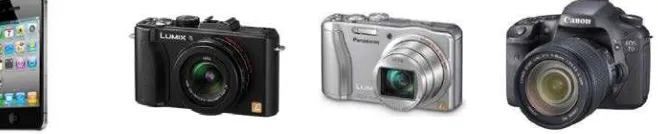
Five different cameras are used in this study (Figure 1). The first camera is a GoPro Hero 1080 with a resolution of 5.04 Mp. The GoPro camera range is a relatively recent creation that is being marketed for many different types of applications, from extreme sports to everyday life. This type of camera is very popular in combination with remote piloted aircraft systems (RPAS) because of their ultra-light weight. However, due to the low-cost camera sensor with a rolling shutter and the fish-eye lens system, the camera is not ideal for photogrammetric work. The second sensor is an in-build camera of an iPhone 4S. The smartphone camera has a resolution of 8 Mp. The main reason for choosing the iPhone was its popularity, as the majority of the population own a smartphone today. They are simplistic in operation and have respectable image properties. The third camera consists of a Panasonic Lumix LX5 with an image resolution of 9.52 Mp. This camera uses a CCD image sensor, which is more expensive to manufacture, but produces a much higher quality image. The camera has a wide perspective, a high quality image sensor and a low distortion Leica lens. All these properties make it the ideal camera for the use with the multi-view 3D reconstruction approach (Thoeni et al., 2012). The fourth camera is a Panasonic Lumix ZS20 which is another point-and-shoot digital camera. It is a high end compact camera with a high image resolution of 14.1 Mp. Nevertheless, this camera is cheaper than the Panasonic Lumix DMC-LX5 because it uses a less expensive CMOS image sensor. The last and fifth camera used in this study presents the professional grade DSLR cameras. It is a Canon E0S 7D with a Canon EF 28 mm lens. This camera has by far the most expensive sensor used in this study. In addition, it has the highest image resolution with 17.92 Mp. At the same time, it seems to be the most complicated camera to use. All relevant technical specifications of the five cameras are listed in Table 1.
2.3 Area of study
The study area is a small rock wall in Pilkington Street Reserve in Newcastle (NSW, Australia), near the Callaghan Campus of the University of Newcastle. The wall is partly smooth with some evident geological features, such as non-persistent joints and
Camera Effective Pixels
*35mm equivalent focal length
Table 1. Important technical specifications of the cameras used in the study
Figure 1. Cameras used in the study (listed according to Table 1)
sharp edges. There is a lot of grass in front of the wall and some on the wall. However, no major bushes or trees are present. The section of the wall taken into account in this study is about 6 m high and 20 m long. Figure 2 shows a textured model of the rock wall.
2.4 Field work and data collection
The first step in the field was to place control point markers on the wall. Eight ground control points (GCP) were evenly placed on the wall. Figure 2 shows their location on the wall with a red circle. The markers consists of a black and with chess board pattern with two black and two white squares each 10 x 10 cm printed on paper (Figure 3). After setting them up, their coordinates where measured by using a reflectorless total station (Leica TPS1205).
The second step consisted in capturing the various images by using the five different cameras. A series of images from each camera was taken. A similar number of images was acquired from a distance of about 5 to 10 m depending on the field of view
of each camera (Table 2).
2.5 Reference model and deviation analysis
The ground truth or reference model was created using a FARO Focus 3D TLS with a range accuracy of ±2 mm. The TLS automatically provides the user with dense point clouds of 3D points. Two scans from two different locations were undertaken in order to improve the accuracy and minimise shadows. The results of the two scans are two dense point clouds with a different reference system. The two point clouds were stitched together using the known locations of the GCPs and other features within the scene. The scan processing software SCENE 3D was used for this purpose. This software provides the user with a wide range of tools to allow for quick and efficient processing. Noise, outliers and duplicated points are automatically detected and removed.
The FARO Focus 3D has an integrated digital camera that is used to capture images of the scene or object in question. This is an automated process that occurs directly after the scanner has scanned the entire scene. These images are used to create point colours in the final 3D models. The final model derived from the laser scan data is shown in Figure 2.
3. DATA PROCESSING
3.1 Camera calibration
The 3D reconstruction pipeline used in Agisoft Photoscan estimates camera calibration parameters automatically utilising Brown's model for lens distortion. In general, this means that manual calibration is not necessary if standard optical lenses and a highly redundant image network are used. For fish-eye lenses such as the one used in the GoPro Hero 1080, the calibration model will fail due to the large radial distortions and due to the large field of view of such lenses. Therefore, Agisoft Lens was used to determine the camera calibration parameters including the non-linear distortion coefficients. These parameters were then input into Photoscan. For all other cameras, auto-calibration was performed using the EXIF camera information found in the images. Figure 2. Reference model obtained with the TLS and locations of the eight GCPs (red circles)
(a) GoPro Hero 1080 (b) Panasonic Lumix LX5
Figure 3. Close-up view of one of the target used for scale and georeferencing
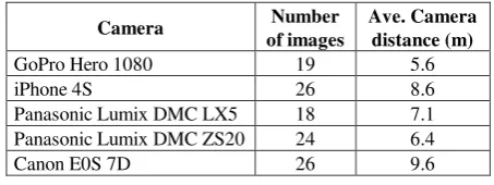
Camera Number
of images
Ave. Camera distance (m)
GoPro Hero 1080 19 5.6
iPhone 4S 26 8.6
Panasonic Lumix DMC LX5 18 7.1
Panasonic Lumix DMC ZS20 24 6.4
Canon E0S 7D 26 9.6
Table 2. Number of images used in the reconstruction process and average camera distance to the wall for each camera
3.2 Scale and georeferencing
Ground control points are added in Agisoft Photoscan through manual selection. This selection process involves creating and placing individual markers on each GCP in each image within the photo set. Markers can be placed before or after an initial alignment. If placing the markers before an initial alignment, the marker positions must be located manually on each image. If an initial alignment is completed before markers have been placed, the software establishes a guided approach to marker placement.
Cameras, such as the GoPro Hero 1080 and the IPhone 4S, have image properties that include a relatively low resolution and consequently a larger pixel size compared to the other cameras. This resulted in increased difficulty when trying to place and match markers on the centre of the targets (Figure 3a). For each image set all GCPs have been selected manually.
3.3 Alignment and optimisation
The alignment process iteratively refines the external and internal camera orientations and camera locations through a least squares solution and builds a sparse 3D point cloud model. Photoscan analyses the source images by detecting stable points and generating descriptors based on surrounding points. These descriptors are later used to align the images by determining the corresponding points in other photographs. The alignment process in Photoscan has a number of parameter controls. There are three different accuracy settings for the alignment process: low, medium and high. The low accuracy setting is useful for obtaining an initial estimate for the camera locations with a relatively short processing time. The high accuracy setting requires much more processing time but camera position estimates obtained would be the most accurate.
An integral result following the alignment process is the estimation of the GCP error values or uncertainty values. These values provide an illustrative representation between the measured GCP coordinates and the estimated GCP coordinates through a least squares solution. During the alignment process using the GCPs, the model is linearly transformed using a 7 parameter similarity transformation (3 parameters for translation, 3 for rotation and 1 for scaling). This kind of transformation between coordinates can only compensate a linear model misalignment. The non-linear component cannot be removed with this approach. This is usually the main reason for GCP
errors. These errors, however, can be minimised using the optimisation tool implemented in Photoscan.
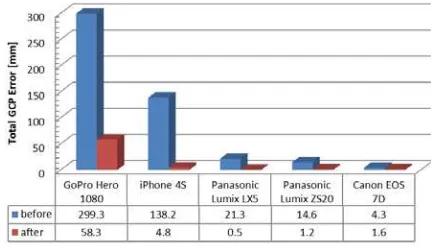
A couple of initial analyses were run in order to find out which alignment accuracy would give good results within a reasonable processing time. The alignment process was executed using all three accuracy measures and the total GCP error was analysed. The initial analyses showed that low accuracy gives the biggest error whereas medium and high accuracy have almost the same error. Therefore, it was decided to run the final models with medium accuracy since processing time is much shorter. Figure 4 shows the total GCP error for the final analyses for all cameras after and before optimisation.
Finally, the influence of the masking option in Photoscan on the GCP accuracy was analysed. Masking is used to remove certain areas or features within each image from the reconstruction process that have the potential to confuse the matching algorithm, and therefore, lead to reprojection errors and result in an inaccurate or incorrect reconstruction. In order to check the influence of masking, the series of images taken with the iPhone 4S were used to build a model using three different options: no masking, background masking, and background and foreground masking (Figure 5). The results are summarised in Table 3, where it can be seen that after optimisation there is little difference. Therefore, it was decided to do the further processing without masking.
(a) no masking (b) background masking
(c) background and foreground masking
Figure 5. The different masking scenarios used for a preliminary error analysis after alignment
Masking Total GCP error (m)
Before after
No masking 0.1382 0.0047
Background masking 0.0773 0.0077
Background and foreground
masking 0.0720 0.0044
Table 3. Influence of masking for results with iPhone 4S before and after optimisation
3.4 Dense point cloud
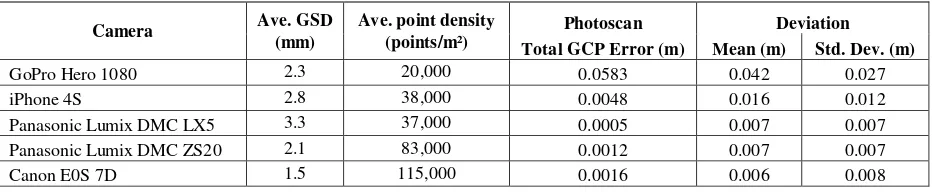
After alignment and optimisation, which included the determination of exterior and interior camera parameters, were complete, the dense multi-view 3D reconstruction algorithm was executed. When exporting a dense point cloud, Photoscan offers the possibility to specify the quality. For this study medium, quality was selected. This resulted in dense point clouds with point cloud densities from 20,000 to over 100,000 points per m2 depending on the camera used.
Figure 4. Total GCP error estimated by Photoscan before and after optimisation for medium alignment accuracy
4. DATA ANALYSIS
Each dense point cloud obtained with Photoscan is compared to the point cloud obtained with the TLS. A deviation analysis is performed where the distance between the two models is calculated. The open-source program CloudCompare is used to perform this analysis. A cloud-to-cloud comparison with a local model is carried out. The Height Field local model was used in order to get the best accuracy for the deviation results. In this model, the reference model is approximated by a mathematical function. The deviation (i.e. the distance) between the TLS model and the image-based model is exactly calculated for each point in the image-based model. The result is a scalar field of the deviation for each image-based model. Before performing the actual deviation analysis, both point clouds were cropped in the same way in order to eliminate any boundary effects.
5. RESULTS AND DISCUSSION
5.1 Results for GoPro Hero 1080
Figure 6 shows the final results of the deviation analysis between the TLS point cloud and the point cloud generated with the GoPro Hero 1080. It can be seen that there are quite a few holes within the scalar field, such as the ones denoted as ‘A’. This is primarily due to Photoscan not being able to fully reconstruct the model. The reasons are not enough redundancy in the images and the loss of definition towards the edge of the ultra-wide angle lens. A visual pixel count in the centre of the photo gives around 2 mm x 2 mm but at the edge it is about 5 mm x 5 mm. The area denoted as ‘B’ exhibits the same surface texture as ‘C’. However, ‘B’ shows very accurate results whereas ‘C’ deviates considerable. Both areas have the same amount of overlapping images but ‘C’ is slightly orientated differently and the camera orientations were not adjusted accordingly. Overall, many areas deviate by 10 cm (red areas) and the mean deviation is around 4 cm. The total GCP error is almost 6 cm, which is considerable considering the scale of the rock wall.
5.2 Results for iPhone 4S
The comparison between TLS data and the model build by using the images from the iPhone 4S is shown in Figure 7. A reasonable good agreement can be observed. The mean deviation is 16 mm and the total GCP error is less than 5 mm. It seems, however, that shade is influencing the results in some areas, as indicated with ‘A’. Nevertheless, the iPhone 4S shows respectful results considering that it is a smartphone people are using every day.
5.3 Results for Panasonic Lumix LX5
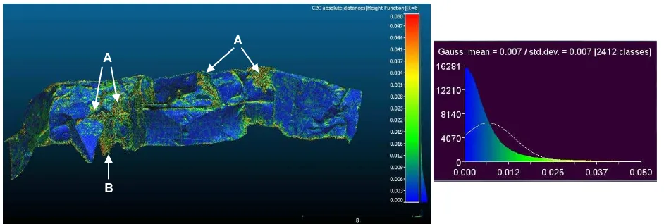
Figure 8 shows the deviation of the model build using the images collected with the Panasonic Lumix LX5. An excellent agreement can be observed. The mean deviation is 7 mm only. The total GCP error is even less than 1 mm, which indicates that the non-linear components of the alignment process could be calculated very accurately during the optimisation process. However, some areas where the model does not totally reflect the same results as obtained by the TLS data can be identified. The deviations in areas such as ‘A’ are related to vegetation. Area ‘B’ has some holes and deviations between 2 and 5 cm. When looking at the images, it can be seen that the images do not have enough overlap. Consequently, the accuracy of the model is decreasing in this area.
5.4 Results for Panasonic Lumix ZS20
Figure 9 summarised the deviation analysis carried out between the TLS data and the model build with the Panasonic Lumix ZS20. The results are very similar to the one obtained with the Panasonic Lumix LX5 (Figure 8). The mean deviation is the same and corresponds to 7 mm. Even the standard deviation is the same with 7 mm. The total GCP error, however, is more than 1 mm. The influence of vegetation can also be seen in areas such as the ones indicated with ‘A’.
5.5 Results for Canon E0S 7D
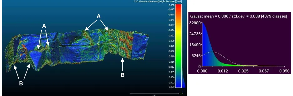
The results of the deviation of the model created using the Canon E0S 7D from the TLS data is shown Figure 10. The results are very similar to the results presented in Figures 8 and 9. The total GCP error is 1.6 mm. The mean deviation is 6 mm only, and therefore, 1 mm smaller than for the Panasonic LX5 and ZS20. However, the standard deviation is 1 mm higher. It can be seen that Figure 10 has more orange and red areas than Figures 8 and 9. Areas with vegetation (‘A’) have also influenced the accuracy. Areas indicated by ‘B’ show some unexpected results. It seems that the deviation in these areas follows a certain pattern which, however, does not correspond to the natural geometry of the rock face. Indeed, Wenzel et al. (2013) observed some similar results and stated that this kind of noise is related to the intersection angle, i.e. the orientation of the camera towards the object. Nevertheless, this behaviour was not observed with any other camera used in this study and the camera orientations and positions were very similar. This means that there could be an additional factor favouring this behaviour.
Camera Ave. GSD
Table 4. Average ground sampling distance (GSD), average point cloud density, total ground control point (GCP) errors from Photoscan and mean and standard deviation of deviation analysis from CloudCompare
A
Figure 6. Error mapping of deviation between TLS and GoPro Hero 1080
Figure 7. Error mapping of deviation between TLS and iPhone 4S
Figure 8. Error mapping of deviation between TLS and Panasonic Lumix LX5 B
C
A A
A
B
A
A
6. CONCLUSIONS
This paper presents a case study which compares results obtained through multi-view 3D reconstruction with data obtained from a TLS. The object of interest is a small rock wall of about 6 m height and 20 m length. Five different digital cameras were used in the study in order to estimate the limits related to the camera type and to establish the minimum camera requirements to obtain comparable results to the ones of the TLS. The cameras used for this study range from commercial grade to professional grade and included a GoPro Hero 1080 (5 Mp), iPhone 4S (8 Mp), Panasonic Lumix LX5 (9.5 Mp), Panasonic Lumix ZS20 (14.1 Mp) and Canon EOS 7D (18 Mp). A series of overlapping images was acquired from a distance of about 5 to 10 m depending on the field of view of each camera. The images were then processed with the commercial software package Agisoft Photoscan in order to obtain a dense point cloud of the rock wall for each camera. Measured control points on the wall were used to scale and georeference the models.
Firstly, it was shown that control points are not only necessary to scale the model but also to compensate for the non-linear model misalignment. Indeed, the accuracy can be considerably improved by using control points and performing the optimisation process in Photoscan. It was also shown that the
total GCP error related to the non-linear model misalignment was major for the GoPro Hero 1080 and the iPhone whereas it was small for the Canon EOS 7D. After optimisation the total GCP error was reduced by a factor of around 20 for most cameras. However, the effect of the non-linear model misalignment could only be completely eliminated for the Panasonic Lumix LX5.
Secondly, the point clouds generated with Photoscan were compared to the point cloud obtained from the TLS. A deviation analysis was carried out with the open-source software CloudCompare where the TLS data was assumed as ground truth. The model based on the images taken with the GoPro Hero 1080 deviated the most, even though the GSD was comparable to the one of the other cameras. One of the reasons is the ultra-wide angle lens. The iPhone 4S showed respectful results considering that it is a smartphone people are using every day. The mean deviation is just 16 mm. However, it seems that shade affected the reconstruction accuracy. The Panasonic Lumix LX5, the Panasonic Lumix ZS20 and the Canon EOS 7D produced comparable results. The analyses showed a mean deviation of 6 to 7 mm with a standard deviation of 7 to 8 mm. Even though the Canon EOS 7D has the highest resolution and is the most expensive camera used in the study, it was shown that the Panasonix Lumix LX5 provided the best results overall, besides Figure 9. Error mapping of deviation between TLS and Panasonic Lumix ZS20
Figure 10. Error mapping of deviation between TLS and Canon EOS 7D A
A
A
A
B
B
having the biggest GSD. The reason is probably the more expensive CCD image sensor.
In conclusion, it can be said that the method of multi-view 3D reconstruction can successfully be applied to model rock faces with sub-centimetre accuracy. There is no need to use very expensive DSLR cameras with very high resolution. An off the shelf compact camera will do the job. However, a rigorous planning for the collection of the images is needed. A highly redundant camera network with overlapping images is required and the orientation of the cameras should be orthogonal to the object whenever possible.
ACKNOWLEDGEMENTS
The authors would like to gratefully acknowledge the assistance provided by their two students Matthew Osborne and James Hord during data collection and data processing. In addition, they would like to acknowledge the financial support of the University of Newcastle (ECR Grant G1300601)
REFERENCES
Agisoft PhotoScan Professional (version 0.9.0),
http://www.agisoft.ru (12 May 2014).
Baltsavias, E.P., 1999. A comparison between photogrammetry and laser scanning. ISPRS Journal of Photogrammetry and
Remote Sensing, 54(2), pp. 83–94.
CloudCompare (version 2.4), http://www.danielgm.net/cc (12 May 2014).
FARO, FARO Focus 3D, http://www.faro.com (12 May 2014).
Favalli, M., Fornaciai, A., Isola, I., Tarquini, S., and Nannipieri, L., 2012. Multiview 3D reconstruction in geosciences.
Computers & Geosciences, 44, pp. 168–176.
Hartley, R., and Zisserman, A., 2003. Multiple view geometry in
computer vision. Cambridge University Press.
Koutsoudis, A., Vidmar, B., Ioannakis, G., Arnaoutoglou, F., Pavlidis, G., and Chamzas, C., 2013. Multi-image 3D reconstruction data evaluation. Journal of Cultural Heritage, 15(1), pp. 73–79.
Snavely, N., Seitz, S. and Szeliski, R., 2006. Photo tourism: Exploring photo collections in 3D. In: Proceedings of SIGGRAPH 2006, pp. 835–846.
Thoeni, K., Irschara, A. and Giacomini A., 2012. Efficient photogrammetric reconstruction of highwalls in open pit coal mines. In: 16th Australasian remote sensing and
photogrammetry conference, pp. 85–90.
Wenzel, K., Rothermel, M., Fritsch, D. and Haala, N., 2013. Image Acquisition and Model Selection for Multi-View Stereo.
International Archives of Photogrammetry. Remote Sensing
and Spatial Information Science, XL-5/W1, pp. 251–258.
Westoby, M. J., Brasington, J., Glasser, N. F., Hambrey, M. J., and Reynolds, J. M., 2012. ‘Structure-from-Motion’
photogrammetry: A low-cost, effective tool for geoscience applications. Geomorphology, 179, pp. 300–314.
Wickens, E. and Barton, N., 1971. The application of photogrammetry to the stability of excavated rock slopes. The
Photogrammetric Record, 7(37), pp. 46–54.