*
GEOMETRIC CALIBRATION OF FULL SPHERICAL PANORAMIC RICOH-THETA
CAMERA
S. Aghayaria*, M. Saadatsereshta, M. Omidalizarandib, I. Neumannb
aFaculty of Surveying and Geospatial Engineering, College of Engineering, University of Tehran, Iran {S.aghayari, msaadat}@ut.ac.ir
b Geodetic Institute, Leibniz Universität Hannover, Germany {zarandi, neumann}@gih.uni-hannover.de
Commission I WG I/9
KEY WORDS: Fisheye Lens, Full Spherical Panorama, Omnidirectional Camera, Network Calibration
ABSTRACT:
A novel calibration process of RICOH-THETA, full-view fisheye camera, is proposed which has numerous applications as a low cost sensor in different disciplines such as photogrammetry, robotic and machine vision and so on. Ricoh Company developed this camera in 2014 that consists of two lenses and is able to capture the whole surrounding environment in one shot. In this research, each lens is calibrated separately and interior/relative orientation parameters (IOPs and ROPs) of the camera are determined on the basis of designed calibration network on the central and side images captured by the aforementioned lenses. Accordingly, designed calibration network is considered as a free distortion grid and applied to the measured control points in the image space as correction terms by means of bilinear interpolation. By performing corresponding corrections, image coordinates are transformed to the unit sphere as an intermediate space between object space and image space in the form of spherical coordinates. Afterwards, IOPs and EOPs of each lens are determined separately through statistical bundle adjustment procedure based on collinearity condition equations. Subsequently, ROPs of two lenses is computed from both EOPs. Our experiments show that by applying 3*3 free distortion grid, image measurements residuals diminish from 1.5 to 0.25 degrees on aforementioned unit sphere.
1. INTRODUCTION
According to the representation of the field of view (FOV), cameras are classified into two main groups: classical cameras with narrow FOV and omnidirectional cameras with very large FOV. Omnidirectional cameras cover the whole surrounding environment and are classified into two categories: Catadioptric (combination of the lenses and mirror) and Dioptric (only lenses) (Micušık, 2004).
Dioptric cameras record the whole front view of the camera mostly with FOV close to 180 degree which is due to having very short focal length. Accordingly, in fisheye images, features distortions increase non-linearly from the center to the sides of the images. Due to having higher resolution in the center of the image with respect to the sides, fisheye lenses and human visual system have similarities (Dhane et al., 2012). This kind of lenses are designed based on fish vision system and have numerous applications in close range photogrammetry and automotive industry (Esparza García, 2015; Hughes et al., 2009; Roulet et al., 2009). For instance, Nissan Motors company developed a system consisting of the four fisheye cameras in four sides of a vehicle for monitoring the surrounding space (Ma et al., 2015). In robotics (Courbon et al., 2007, 2012), space mission (Suda and Demura, 2015) or mobile mapping system (e.g. texturizing the point clouds of terrestrial laser scanner), a few fisheye images are enough to be captured instead of numerous normal lens images (Brun et al., 2007)
.
Utilizing fisheye camera in aforementioned applications is restricted by presence of large distortions (i.e. straight lines appear as curve lines). Consequently, camera calibration is a pre-requisite step and a fundamental issue forfurther scientific and photogrammetric tasks feature extraction from images or 3D reconstruction.
In classical cameras, a pinhole camera model with normal lens distortion model is quite good enough to approximate projection ray into the image plane. However, this model is not appropriate for fisheye lens images due to limitation of perspective projection in increasing incidence angle rays relative to the optical axes. Hence, unlike the classical perspective cameras, these kinds of cameras do not follow perspective projection. Equation 1 depicts the perspective projection as follows:
ݎ୮ୣ୰ୱ୮ୣୡ୲୧୴ୣൌ ݂ݐܽ݊ሺሻ (1)
where r = radial distance from perspective centre f = focal length
= angle between incoming ray and principal axis In perspective projection, rays are straight lines and intersect in the projection centre, but fisheye images are defined based on specific projection equations as follows: (Kannala and Brandt, 2006; Schneider et al., 2009).
ݎୱ୲ୣ୰ୣ୭୰ୟ୮୦୧ୡൌ ʹ݂ݐܽ݊ሺȀʹሻ (2)
ݎୣ୯୳୧ୢ୧ୱ୲ୟ୬ୡୣൌ ݂ (3)
ݎୣ୯୳୧ୱ୭୪୧ୢൌ ʹ݂ݏ݅݊ሺȀʹሻ (4)
Equations 2 to 5 are known as stereographic projection, equidistance projection, equisolid angle projection and orthogonal projection respectively.
Perhaps the common projection to design the fisheye camera is equidistance projection (Kannala and Brandt, 2006; Schneider et al., 2009).
Several calibration models have been proposed for these types of lenses. The solution by Suda and Demura ( 2015) is based on rewritten equations 2 to 5 with coefficients of radial distortion. Ma et al. (2015) proposed an approach based on spherical projection that points are projected to the unit sphere and epipolar geometry 3D reconstruction is carried out. In Hughes et al. (2010) approach, straight lines become part of circles with different radius in fisheye images. Vanishing points are intersections of these arcs and the lines are defined by these two points going through the distortion center. Afterwards, calibration is performed according to the distortion center and the proposed mathematical model. Schneider et al. (2009) developed four geometric models for fisheye lenses based upon stereographic, equidistance, equisolid and orthogonal projection geometry to project object points to images and they added additional parameters to calibrate the images that are captured from a 14 Megapixel camera equipped with Nikkon 8 mm fisheye lens. Zhang et al. (2015) proposed an approach based on the extraction of arcs in fisheye images. Rectification is performed to generate perspective images using curvatures to estimate intrinsic calibration parameters that consist of focal length, image center and aspect ratio. Wang et al. (2014) investigated two camera models to calibrate fisheye lens (pinhole camera model and spherical projection model) to show that spherical camera projection model works more precisely and more efficiently for the non-linear image system. Dhane et al. (2012) performed direct mapping from fisheye image to perspective image and consequently applied inverse mapping from corrected image to fisheye image for correcting these kind of images. Proposed methodology is online and has the ability to run on DSP and FPGA platform. Kannala and Brandt (2006) proposed a calibration method on the basis of generic camera model and used planar calibration pattern with control points to estimate IOPs and EOPs parameters. In this research, a novel geometric calibration of full spherical image is presented. Calibration procedure is performed on the unit sphere. IOPs are defined for defined network points (Figure 5) and subsequently added to the measured control points in image space as correction terms to be considered in collinearity equations, in the form of spherical coordinate systems, to obtain direction vectors between image points and object points. The EOPs and IOPs are determined through collinearity equations of spherical coordinates via statistical bundle adjustment procedure. Then ROPs are calculated from both EOPs of central and side lenses.
In the following section, the specification of the used camera for calibration is represented. In section 3, developed mathematical calibration model for the fisheye lens is discussed. In section 4, hemispherical calibration room and the precision of control points in both object and image spaces are investigated. Experimental results are presented in section 5 and the summary and conclusions are represented and discussed in section 6.
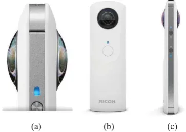
2. CAMERA SPECIFICATIONS In order to take fully spherical photographs, many panoramic cameras composed of classical or fisheye lenses can be utilized in the camera system (Rau et al., 2016). These cameras need to be synchronized to create full spherical view by stitching images together which is a time consuming procedure. Ricoh Company developed a camera in 2014 that is able to capture the whole surrounding environment in one shot and is known as RICOH-THETA (Ricoh, 2016). This camera consists of two lenses (Figure 1) which cover the entire scene by 360*180 degrees. The images are stitched together using embedded software inside the camera and there is no possibility to access raw images in current version of camera. Therefor stitching images errors remain unknown and cannot be obtained throughout adjustment procedure.
(a) (b) (c) Figure 1. Ricoh-Theta Camera. (a) Magnification of the two
fisheye lenses in side view, (b) cameras front view and (c) side view. Calibration procedure of each lens is performed separately and it starts by defining three spaces as follows:
1- Image space 2- Unit sphere space 3- Object space
(b) (c)
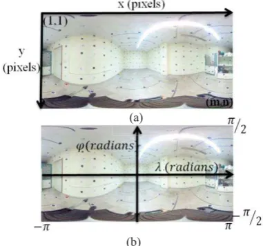
Figure 2. (a) Full spherical image, (b) central image (i.e. front lens), (c) side image (i.e. back lens).
3.1 From image space to unit sphere space
Image coordinates (x, y) are moved to spherical coordinate system by equirectangular projection (Equations 6 and 7). Both coordinate systems are represented in Figure 3.
(b)
Figure 3. Coordinate systems, (a) image space coordinate system in pixel unit, (b) spherical coordinate system in radian
unit.
ߣ ൌ ቀݔ െ݊ʹቁ Ǥʹߨ݊ (6)
߮ ൌ ቀ݉ʹ െ ݕቁ Ǥ݉ߨ (7)
where x, y = image space coordinates in pixels ߮,ߣ= latitude and longitude in radians m, n = image size in pixels
From the illustrations of coordinate systems in figure 3, the image size (height and width) in spherical coordinate system is equal to (ߨǡ ʹߨሻǤFrom equations 8 and 9, relation n=2m is proved.
ͳ ൏ ݔ ൏ ݊ܽ݊݀ͳ ൏ ݕ ൏ ݉ (8)
െߨ ൏ ߣ ൏ ߨܽ݊݀ െ ߨ ʹൗ ൏ ߮ ൏ ߨ ʹൗ ܽ݊݀ (9) Transformation of spherical coordinate system to unit sphere space is performed based on equation 10.
ቈݔݕ ݖ ൌ
ሺ߮ሻ Ǥ ሺߣሻ ሺ߮ሻ Ǥ ሺߣሻ
ሺ߮ሻ (10)
3.2 From world space to unit sphere space
By applying Helmert transformation (three rotations, three translations and one scale) world coordinate system is transformed to unit sphere based on equation 11. (Vectors and matrices are representing in boldface and scalars are represented as non-bold typeface).
࢞ൌ ߤǤ ࡾሺࢄെ ࢀሻ (11) where xi = unit sphere coordinate system [x, y, z] of ith point
ߤ = scale of ith point = norm (Xi-T)-1 ࡾ= 3*3 rotation matrix
ࢀ= translation matrix [ܶ௫ǡ ܶ௬ǡ ܶ௭ሿԢ
Xi = world coordinates ሾܺǡ ܻǡ ܼሿԢ of ith point
In the next section, IOPs are discussed and presented to take them into account for deriving the final equation.
3.3 Interior orientation parameters (IOPs)
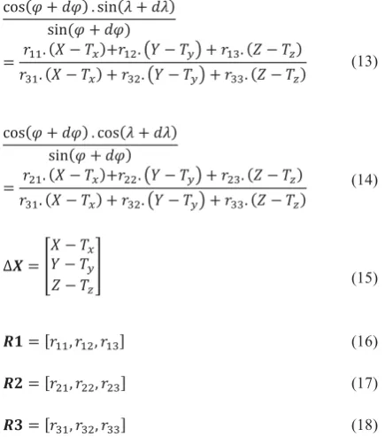
In an ideal case of the calibration procedure, there is an assumption that unit sphere center, points on unit sphere and their object coordinates lie on the same line as a direction vector (i.e. collinearity equations). Figure 4 depicts an uncorrected point on unit sphere that needs to be calibrated to lie on the same line. In other words, by transferring the image and object points to unit sphere, these points can coincide. However in reality, the points on unit sphere need corrections with respect to the direction vector. Thus, ݀ߣ and ݀߮ are defined as IOPs parameters in equation 12 as follows:
ሺ߮ ݀߮ሻ Ǥ ሺߣ ݀ߣሻ ሺ߮ ݀߮ሻ Ǥ ሺߣ ݀ߣሻ
ሺ߮ ݀߮ሻ
ൌ ߤǤ ࡾǤ ܺ െ ܻܶ െ ܶ௬௫
ܼ െ ܶ௭
(12)
Figure 4. Ideal line (blue) where three points lie on the same line versus uncalibrated situation (red).
(a)
The scale parameter leads to instability of estimated parameters and should be removed from equation 12. For this purpose, first and second rows are divided by third row which comes to collinearity equation in the form of spherical coordinate system.
ሺ߮ ݀߮ሻ Ǥ ሺߣ ݀ߣሻ ሺ߮ ݀߮ሻ
ൌ ݎଵଵǤ ሺܺ െ ܶ௫ሻݎଵଶǤ ൫ܻ െ ܶ௬൯ ݎଵଷǤ ሺܼ െ ܶ௭ሻ ݎଷଵǤ ሺܺ െ ܶ௫ሻ ݎଷଶǤ ൫ܻ െ ܶ௬൯ ݎଷଷǤ ሺܼ െ ܶ௭ሻ
(13)
ሺ߮ ݀߮ሻ Ǥ ሺߣ ݀ߣሻ ሺ߮ ݀߮ሻ
ൌ ݎଶଵǤ ሺܺ െ ܶ௫ሻݎଶଶǤ ൫ܻ െ ܶ௬൯ ݎଶଷǤ ሺܼ െ ܶ௭ሻ ݎଷଵǤ ሺܺ െ ܶ௫ሻ ݎଷଶǤ ൫ܻ െ ܶ௬൯ ݎଷଷǤ ሺܼ െ ܶ௭ሻ
(14)
οࢄ ൌ ܺ െ ܻܶ െ ܶ௬௫
ܼ െ ܶ௭
(15)
ࡾ ൌ ሾݎଵଵǡ ݎଵଶǡ ݎଵଷሿ (16)
ࡾ ൌ ሾݎଶଵǡ ݎଶଶǡ ݎଶଷሿ (17)
ࡾ ൌ ሾݎଷଵǡ ݎଷଶǡ ݎଷଷሿ (18) With consideration of equations 13 to 18, equations 19 and 20 are obtained.
ܨǣ ሺߣ ݀ߣሻǤ ሺࡾǤ οࢄሻ െ ሺ߶
݀߮ሻǤ ሺࡾǤ οࢄሻ ൌ Ͳ (19) ܩǣ ሺߣ ݀ߣሻǤ ሺࡾǤ οࢄሻ െ ሺ߶
݀߮ሻǤ ሺࡾǤ οࢄሻ ൌ Ͳ (20)
Number of unknown parameters and equations in central image for M control points are computed as follows:
Unknowns: ሺʹ כ ܯሻሼܫܱܲݏሽ ሼܧܱܲݏሽ
Equations: ʹ כ ܯ
In this case, for each image point two correction terms are defined as IOPs with respect to corresponding control point and six EOPs parameters. This linear system is under-determined due to the fact that the numbers of equations are less than the number of unknowns. To deal with this problem, nine networks are considered on the image and vertices of this network are obtained by bilinear interpolation. Figure 5 shows nine networks on the central image. In the calibration procedure, the vertices of each network are assumed as IOPs and coordinates of some other image points in central image are calculated by means of bilinear interpolation of vertices of corresponding network. This procedure is also repeated for side image as well. As an exemplary case here, we have nine networks in the central image which include 100 control points; hence the number of unknowns and equations are:
Unknown: ʹ כ ͳͲሼܫܱܲሽ ሼܧܱܲሽ ൌ ʹ
Equations: ʹ כ ͳͲͲ ൌ ʹͲͲ
Consequently, ten ݀ߣ and ten ݀߮ are obtained as network vertices for each image. It is important to notice that in
equirectangular plane, four vertices of distortion-free grids in the north or south poles (first or last rows) have the same values and considered as one unique point. By considering Figure 5 for network 1, equations 19 and 20 are changed to equations 21 and 22.
ܨǣ ൫ߣ ሺሺܽଵǤ ݀ߣଵ ܽଶǤ ݀ߣଵ
ܽଷǤ ݀ߣଶ ܽସǤ ݀ߣଷሻ൯ Ǥ ሺࡾǤ οࢄሻ െ
൫߶ ሺܽଵǤ ݀߮ଵ ܽଶǤ ݀߮ଵ
ܽଷǤ ݀߮ଶ ܽସǤ ݀߮ଷሻ൯ Ǥ ሺࡾǤ οࢄሻ ൌ Ͳ
(21)
ܩǣ ൫ߣ ሺܽଵǤ ݀ߣଵ ܽଶǤ ݀ߣଵ
ܽଷǤ ݀ߣଶ ܽସǤ ݀ߣଷሻ൯ Ǥ ሺࡾǤ οࢄሻ െ
൫߶ ሺܽଵǤ ݀߮ଵ ܽଶǤ ݀߮ଵ
ܽଷǤ ݀߮ଶ ܽସǤ ݀߮ଷሻ൯ Ǥ ሺࡾǤ οࢄሻ ൌ Ͳ
(22)
where ߮,ߣ= latitude and longitude
݀ߣଵݐ݀ߣଷ= longitude of the first network (IOP) ݀߮ଵݐ݀߮ଷ= latitude of the first network (IOP) a1 to a4 = bilinear coefficients of the four corners
a1 to a4 are defined for each point inside the network as bilinear coefficients and they are the same for ݀ߣ and ݀߶.
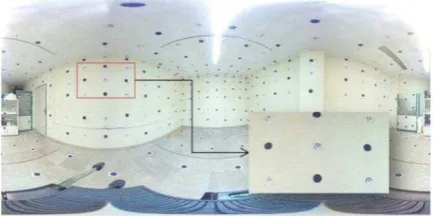
Figure 5. Representation of nine networks on the central image.
3.4 Relative Orientation Parameters (ROPs)
In addition to IOPs of each lens, the second group of camera calibration parameters are relative position and rotation of both lenses named ROPs. The ROPs can be computed from EOPs of both lenses by relation 23 and 24.
ࢄ ൌ ࡾଵࢄଵ ࢀଵൌ ࡾଶࢄଶ ࢀଶ՜
ࢄଶൌ ࡾଶ்ሺࡾଵࢄଵ ࢀଵെ ࢀଶሻ
(23)
ࡾோைൌ ࡾଶ்ࡾଵܽ݊݀ࢀோைൌ ࡾଶ்ሺࢀଶെ ࢀଵሻ (24)
In which EOPi=[RiTi] for i=1:2 for each lens.
Throughout the adjustment procedure, global and local tests are performed for each type of observation to reject outliers based on chi-square statistical test with confidence level of 99.7 percent. This procedure continues until no measurements remain to be rejected (Omidalizarandi and Neumann, 2015; Omidalizarandi et al., 2016).
3.5 Initialization of EOPs and IOPs
ࢄ ൌ ݏǤ ࡹǤ ࢞ ࢀ௫ (25) where s =1/ߤ
M =R-1
Homogenous representations of coordinates are represented in equations 26 and 27 as follows:
൦ translations and one scale, while A is the coefficient matrix. In this step, translations are just calculated by singular value decomposition (SVD).
SVD for matrix A is defined as follows (Khoshelham, 2016):
ሾࡿǡ ࢂǡ ࡰሿ ൌ ܸܵܦሺሻ ՜ ൌ ࡿǤ ࢂǤ ࡰ் (28) each control points is calculated based on equation 29.
ߣൌ ටሺܺെ ܶ௫ሻଶ ൫ܻെ ܶ௬൯ଶ ሺܼെ ܶ௭ሻଶ (29)
Afterwards rotations are calculated from equations 30 and 31 by considering equation 25.
ሺࢄ െ ࢀ௫ሻ ൌ ࡹǤ ሺݏǤ ࢞ሻ (30)
ࡹ ൌ ൫ሺݏǤ ࢞ሻᇱכ ሺݏǤ ࢞ሻ൯ିଵ
כ ൫ሺݏǤ ࢞ሻᇱכ ሺࢄ െ ࢀ௫ሻ൯ (31) For further information regarding decomposition of rotation matrix, please refer to work of Förstner and Wrobel (2016).
4. Calibration room
The calibration room is located in the Photogrammetric Institute of University of Tehran and it is covered with known 3D control points. These points are well distributed around the calibration room which fully cover the whole spherical image (figure 6). Image coordinates of these points are extracted using PhotoModeler software (PhotoModeler, 2016) Targets centroid are principally extracted based on least squares ellipse fitting. Object points are measured by Leica Flex Line TS06 plus (Leica, 2016) in local coordinate system with accuracy of 2 mm+2 ppm in distance measurement and 1 second in angle measurement. Table 1 shows the standard deviations of object coordinates. As a disadvantage of this type of camera is capturing wide FOV images with low resolution which directly influencing on the image quality. Accordingly, target centroid detection becomes a challenging issue in image space. To overcome this problem, targets are designed in large size (i.e. diameters of 8 centimetres) to be visible in the captured images.
Furthermore, in this research, all extracted target centroids have the same accuracy throughout the adjustment procedure.
σ ܺ(mm) σ ܻ(mm) σ ܼ(mm)
Mean
Max 0.981.99 1.552 0.948.42
Table 1. Statistics of the object point standard deviations.
Figure 6. Illustration of targets in calibration room. 5. Experimental results
As mentioned previously, each lens is calibrated separately. Dataset 1 consists of 107 and 78 and dataset 2 consist of 125 and 60 control points in central and side images respectively. Table 2 shows the calibration parameters of central and side image. In this research, calibration is performed for nine networks on image; therefore we have ten ∆φ and ten ∆λ in unit sphere as IOPs.
To obtain IOPs, firstly, Initial IOPs are considered zero and EOPs are calculated based on SVD according to section 3.5. Then the algorithm detects corresponding network for each control point. Finally, IOPs and EOPs are computed on the basis of rigorous statistical bundle adjustment procedure with applied Gauss-Helmert model to update observations and estimating unknowns throughout the adjustment procedure., In addition, since the minimum accuracy of the target measurements in the object space is 2mm, consequently the calibration quality is decreased.
Points with large residuals are discarded in both image and object spaces by means of chi-square test with 99.7% level of confidence. Table 3 shows the EOPs of each lens and PORs between them. Differences between values show that the lenses have their own coordinate system with different orientation even though they stick together to create full spherical images. Merely considering unique IOPs and EOPs for both central and side images leads to increasing residuals, separates the calibration of lenses and significantly decreases residuals in the calibration procedure.
to random vectors after calibration. It means that the calibration process has been successful performed to model image distortions.
Dataset1 Dataset2 Central image IOPs
οߣଵ ο߮ଵ -1.18503 0.12296 -1.45378 0.11901
οߣଶ ο߮ଶ -1.46116 0.06972 -1.67114 0.00357
οߣଷ ο߮ଷ -1.07494 0.12452 -1.47210 0.12651
οߣସ ο߮ସ -0.67197 -0.08979 -1.03064 -0.02593
οߣହ ο߮ହ -0.84415 -0.19812 -1.17575 -0.13754
οߣ ο߮ -1.55720 -0.18099 -1.70940 -0.22682
οߣ ο߮ -1.15013 -0.43468 -1.47118 -0.43483
οߣ଼ ο଼߮ -0.74798 -0.26941 -1.03435 -0.25386
οߣଽ ο߮ଽ -0.96754 -0.05133 -1.14622 0.09077
οߣଵ ο߮ଵ -1.3880 0.055168 -1.70744 -0.00772 Side image IOPs
οߣଵ ο߮ଵ -0.51068 0.36832 -0.11075 0.08239
οߣଶ ο߮ଶ -0.06341 -0.98527 0.50886 -0.71481
οߣଷ ο߮ଷ -0.40143 -0.23769 -0.36806 -0.14972
οߣସ ο߮ସ 0.37308 0.38276 0.53805 0.32361
οߣହ ο߮ହ -0.17277 0.57052 0.25259 0.53938
οߣ ο߮ -0.04106 -0.63212 0.53608 -0.38344
οߣ ο߮ 0.09680 -0.65990 -0.13101 -0.69211
οߣ଼ ο଼߮ 0.50846 -0.10731 0.81087 -0.21124
οߣଽ ο߮ଽ -0.43738 0.38495 0.22173 0.43706
οߣଵ ο߮ଵ 0.40035 0.17699 0.66018 0.01718 Table 2. Calibration parameters of side and central image, οߣ
and ο߮ in degree unit for two datasetes.
EOPs Central image imageSide ROPs
Dataset Table 3. EOPs of each lens and ROPs between them.
6. Summary and conclusions
In this research, a novel full spherical RICOH-THETA camera calibration is developed and discussed. The aforementioned camera consists of two lenses which are calibrated separately. Calibration is carried out in intermediate space between image and object space that is called unit sphere space in this research. First, the coordinates are transferred from image space to unit sphere by equirectangular projection. Measured control points are transformed to unit sphere by considering two correction terms of IOPs. Subsequently, two collinearity equations in Since unknown parameters (IOPs + EOPs) become more than the equations (under determined), a distortion-free grid with nine cells is designed on the images to reduce unknown parameters.
the form of spherical coordinate system are defined by considering the EOPs (six parameters).
EOPs are determined based upon Helmert transformation and it projects coordinates from object space to unit sphere. Then ROPs are computed from both EOPs.
SVD is performed to compute initial EOPs. A rigorous statistical bundle adjustment is implemented to optimally calculate the parameters. Outliers and large residuals are discarded by applying chi-square test with 99.7% level of confidence. Results show that maximum residuals of coordinates in central and side image for dataset 1 are 0.15 and 0.26 degrees and for dataset 2 are 0.14 and 0.24 degrees respectively.
The proposed model is a mathematical model which consists of all errors like stitching error, affine error, redial symmetric and tangential errors and etc. There is no way to access some of these errors such as stitching error in images that cause difficulty in calculating some other errors like radial symmetric by proposed approach.
7. Future Works
By increasing the number of grids, depending on the distribution of the control points on the captured images, some girds remain without control points that lead to zero columns in design matrix. By increasing the number of grids, the number of zero columns increased, and therefore it decreases its rank and causes singularity. For this reason, some equations should be considered as constraints, and in this step, optimum number of grids is a challenging issue. Another approach is an analytical model which can be used instead of grids. But in this case, the challenge is related to the optimum model.
By overcoming aforementioned challenges, systematic errors on the central image are determined (IOPs in Table 2 for fisheye camera. Mobile Mapping Technologies, Padoue, Italie, pp. 29–31.
Courbon, J., Mezouar, Y., Eckt, L., and Martinet, P. (2007). A generic fisheye camera model for robotic applications. In 2007 IEEE/RSJ International Conference on Intelligent Robots and Systems, pp. 1683–1688.
Courbon, J., Mezouar, Y., and Martinet, P. (2012). Evaluation of the Unified Model of the Sphere for Fisheye Cameras in Robotic Applications. Advanced Robotics 26,
947–967.
(a) (b)
(c) (d)
(e) (f)
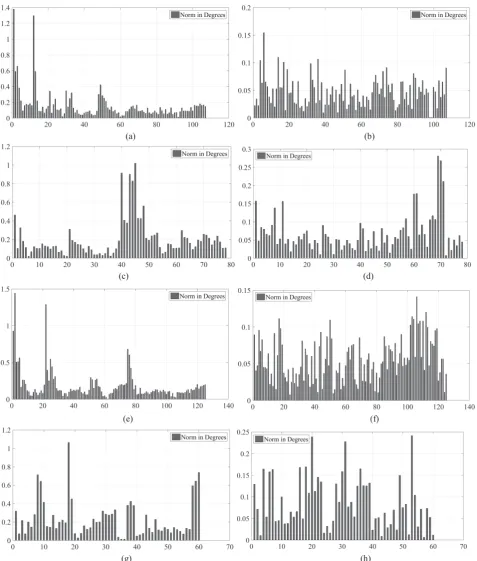
(g) (h)
Figure 7. Norm of λ and φ residuals of each control points before (a, c, e and g) and after (b, d, f and h) camera calibration, (a) central image residuals of dataset 1 befor calibration and (b) after calibration, (c) side image residuals of dataset 1 befor calibration and (d) after calibration, (e) central image residuals of dataset 2 befor calibration and (f) after calibration, (g) side image residuals of dataset
(a) (b)
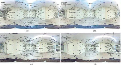
(c) (d)
Figure 8. Residuals vector of all control points in image space before (a and c) and after (b and d) calibration for dataset1 (a and b) and dataset 2 (c and d).
Dhane, P., Kutty, K., and Bangadkar, S. (2012). A generic non-linear method for fisheye correction. International Journal of Computer Applications 51, pp. 58-65
Förstner, W., and Wrobel, B.P. (2016). Photogrammetric computer vision: statistics, geometry, orientation and reconstruction. (Springer International Publishing). ISSN 1866-6795, volume 11, pp. 330-331.
Hughes, C., Glavin, M., Jones, E., and Denny, P. (2009). Wide-angle camera technology for automotive applications: a review. IET Intelligent Transport Systems 3, 19–31.
Hughes, C., McFeely, R., Denny, P., Glavin, M., and Jones, E. (2010). Equidistant (Fθ) Fish-eye Perspective with Application in Distortion Centre Estimation. Image Vision Comput. 28, 538–551.
Kannala, J., and Brandt, S.S. (2006). A generic camera model and calibration method for conventional, wide-angle, and fish-eye lenses. IEEE Transactions on Pattern Analysis and Machine Intelligence 28, 1335–1340.
Khoshelham, K. (2016). Closed-form solutions for estimating a rigid motion from plane correspondences extracted from point clouds. ISPRS Journal of Photogrammetry and Remote Sensing 114, 78–91.
Leica (2016). Leica FlexLine TS06plus Manual Total Station. [Online]. Available: http://leica-geosystems.com /en/products/total-stations/manual-total-stations/leica-flexline-ts06plus [Accessed: 20-Nov-2016].
Ma, C., Shi, L., Huang, H., and Yan, M. (2015). 3D Reconstruction from Full-view Fisheye Camera. Computer
Vision and Pattern Recognition (cs.CV). arXiv:1506.06273 [Cs].
Micušık, B. (2004). Two-view geometry of omnidirectional cameras. Czech Technical University in Prague. PHD thesis.
Omidalizarandi, M., and Neumann, I. (2015). Comparison of Target- and Mutual Information based Calibration of Terrestrial Laser Scanner and Digital Camera for Deformation Monitoring. The International Archives of Photogrammetry, Remote Sensing and Spatial Information Sciences 40, 559-564.
Omidalizarandi, M., Paffenholz, J.-A., Stenz, U., and Neumann, I. (2016). Highly Accurate Extrinsic Calibration of Terrestrial Laser Scanner and Digital Camera for Structural Monitoring Applications. 3rd Joint International Symposium on Deformation Monitoring (JISDM), CD-proceedings
PhotoModeler (2016). PhotoModeler - close-range photogrammetry and image-based modeling. [Online]. Available: http://www.photomodeler.com/index.html. [Accessed: 20-Nov-2016].
Rau, J.Y., Su, B.W., Hsiao, K.W., and Jhan, J.P. (2016). Systematic Calibration for a Backpacked Spherical Photogrammetry Imaging System. ISPRS-International Archives of the Photogrammetry, Remote Sensing and Spatial Information Sciences, pp. 695–702.
Ricoh (2016). Spherical Imaging Device | Global | Ricoh. [Online]. Available: http://www.ricoh.com/technology /tech/065_theta.html. [Accessed: 13-Nov-2016]
Roulet, P., Konen, P., and Thibault, S. (2009). Multi-task single lens for automotive vision applications. In SPIE
0.2 Degrees 0.2 Degrees
Defense, Security, and Sensing, (International Society for Optics and Photonics), pp. 731409–731409.
Schneider, D., Schwalbe, E., and Maas, H.-G. (2009). Validation of geometric models for fisheye lenses. ISPRS Journal of Photogrammetry and Remote Sensing 64, 259–
266.
Suda, R., and Demura, H. (2015). Calibration Tools of Fish-Eye Cameras for Monitoring/Navigation in Space Missions. In Lunar and Planetary Science Conference, pp. 1767-1768.
Wang, K., Zhao, L., and Li, R. (2014). Fisheye omnidirectional camera calibration #x2014; Pinhole or spherical model? In 2014 IEEE International Conference on Robotics and Biomimetics (ROBIO), pp. 873–877.