RECONSTRUCTING WHITE WALLS:
MULTI-VIEW, MULTI-SHOT 3D RECONSTRUCTION OF TEXTURELESS SURFACES
Andreas Ley, Ronny H¨ansch, Olaf Hellwich
Computer Vision & Remote Sensing Group, Technische Universit¨at Berlin, Berlin, Germany (andreas.ley, r.haensch, olaf.hellwich)@tu-berlin.de
KEY WORDS:Structure from Motion, Multi-View Stereo, 3D Reconstruction, Image Enhancement, Denoising
ABSTRACT:
The reconstruction of the 3D geometry of a scene based on image sequences has been a very active field of research for decades. Nevertheless, there are still existing challenges in particular for homogeneous parts of objects. This paper proposes a solution to enhance the 3D reconstruction of weakly-textured surfaces by using standard cameras as well as a standard multi-view stereo pipeline. The underlying idea of the proposed method is based on improving the signal-to-noise ratio in weakly-textured regions while adaptively amplifying the local contrast to make better use of the limited numerical range in 8-bit images. Based on this premise, multiple shots per viewpoint are used to suppress statistically uncorrelated noise and enhance low-contrast texture. By only changing the image acquisition and adding a preprocessing step, a tremendous increase of up to300%in completeness of the 3D reconstruction is achieved.
1. INTRODUCTION
The reconstruction of the 3D geometry of a scene based on im-age sequences has been a very active field of research. The joint effort in the development of keypoint detectors, matching tech-niques, path estimation methods, bundle adjustment, and dense reconstruction has resulted in very successful solutions that are able to robustly and accurately reconstruct a 3D scene from given images. Nevertheless, there are still existing challenges in partic-ular for difficult acquisition circumstances (e.g. inhomogeneous or nonconstant lighting), difficult objects (e.g. with homogeneous or reflective surfaces), or certain application scenarios (e.g. fa-cade reconstruction). One especially critical example are weakly-textured parts of objects, where the lack of correct matches leads to holes and topological errors within the 3D point cloud.
This paper proposes to enhance the 3D reconstruction of weakly-textured surfaces by using standard cameras as well as a standard multi-view stereo (MVS) pipeline. Only changing image acqui-sition and adding a preprocessing step enabled a tremendous in-crease in completeness of the achieved reconstruction.
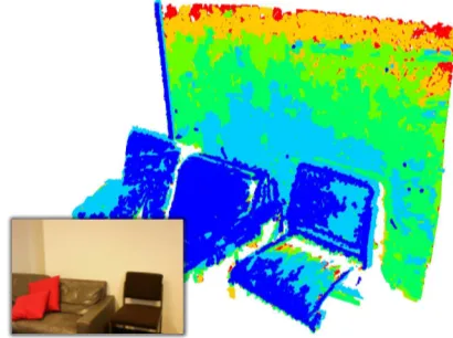
The underlying idea of the proposed method is based on the in-sight that in the real world there is no such thing as a textureless surface. What is usually meant with this phrase is that the exist-ing physical texture is either too fine-grained to be captured by the spatial resolution of a given camera, or that it has insufficient contrast. Especially the latter causes the contribution of the phys-ical texture to the measured signal to drop below the contribution of the measurement noise, which makes a distinction of the two close to impossible. Consequently, all that is necessary to exploit the existing texture in this case is to enhance the signal-to-noise-ratio. Based on this premise, this paper proposes to use multiple shots per viewpoint to suppress statistically uncorrelated noise and enhance low-contrast texture. It models the measured signal as a mixture of truly random as well as fixed-pattern noise and leads to a significant improvement of image quality and (more importantly) of the completeness of the reconstruction. An ex-ample is shown in Figure 1, where 3D points are color coded depending on how many images per viewpoint were at least nec-essary for their reconstruction (1 ˆ=blue to 30 ˆ=red). A flexible and open-source C++ implementation of the proposed framework is publicly available (Ley, 2016).
Figure 1. Exemplary reconstruction: 3D points are color coded depending on how many images per viewpoint were at least nec-essary for their reconstruction (1 ˆ=blue to30 ˆ=red)
2. RELATED WORK
The principle idea to increase the image quality to ease the task of 3D reconstruction is not new. Previous approaches can be coarsely divided into two groups: Exploiting multiple images or using local enhancement methods based on a single image.
Only few works try to exploit the advantages of HDR images for computer vision applications in general and multi-view stereo in particular. The advantages of HDR photogrammetry have been shown in laboratory experiments in (Cai, 2013). While HDR im-ages are used in (Ntregkaa et al., 2013) and (Guidi et al., 2014) to improve 3D reconstructions by simultaneously enhancing con-trast in dark and bright regions of buildings and vases/plates of cultural heritage, respectively, (Kontogianni et al., 2015) investi-gates the influence of HDR images on keypoint detection.
It might not be possible or desirable in all cases to acquire multi-ple images from the same viewpoint or to rely on more advanced HDR image composition techniques that can handle moving cam-eras. The next best choice is to use contrast enhancement tech-niques that are based on a single image. It has been shown that contrast enhancement increases the performance of keypoint de-tectors (e.g. (Lehtola and Ronnholm, 2014)). The work of (Bal-labeni et al., 2015) investigates the influence of multiple image preprocessing techniques including color balancing, image de-noising, RGB to gray conversion, and content enhancement on the performance of the 3D reconstruction pipeline.
3. PROPOSED METHODOLOGY
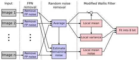
Weakly-textured areas in images generally pose two crucial prob-lems for any 3D reconstruction pipeline. First, as discussed above, “textureless” often means that the texture is “hidden” because the contribution of the physical texture to the measured signal is ap-proximately as strong as the measurement noise. Consequently, the first task is to enhance the signal, i.e. to significantly suppress the noise. The second problem is that the restored texture remains weak compared to image areas with higher contrast but needs to be stored within the same image data. HDR images for example solve this problem by allowing enough numerical precision to si-multaneously represent small and large signal changes. However, freely available MVS pipelines that can process HDR images (or similar advanced formats) are rare ((Rothermel et al., 2012) is one of the few exceptions). That is why the second task consists of saving weak and strong texture components within the same8 -bit image to use common reconstruction software. An overview of the proposed noise reduction is visualized in Figure 2.
Image 2
Image 1 Remove
FP noise
Image n
...
Remove FP noise
Remove FP noise
Average
Estimate remaining
noise
Local mean
Local variance
Local mean noise
Fit into 8 bit
-+
Input FPN removal
Random noise removal
Modified Wallis Filter
...
Figure 2. Flowchart of the proposed method
To actually increase the signal-to-noise ratio (SNR) we explore the idea of averaging multiple images per viewpoint. The photog-rapher is required to take a whole range of images per viewpoint by shooting with a tripod to guarantee alignment. The images are averaged to suppress the stochastic noise. In theory this should result in a reduction of the noise’s standard deviation by1/√nfor nimages under the assumption of iid. noise. The combination of multiple exposures into a single image is similar to the HDR ra-diance acquisition proposed by e.g. (Debevec and Malik, 1997) which was shown to improve 3D reconstructions with under- and overexposed regions (Guidi et al., 2014). Contrary to (Guidi et al., 2014) we do not try to acquire as few images per viewpoint as
possible while covering a large exposure range. Instead we use a large batch of images per viewpoint covering a small exposure range, which can easily be accomplished with extended camera firmwares that support scripting.
The approach of averaging can only deal with random fluctua-tions that are temporally decorrelated. Realistic image noise is more complicated than that and is actually a mixture of this spa-tially and temporally random process and a spaspa-tially random but temporally deterministic process (i.e. fixed pattern noise, FPN). We model both effects by an extended signal model (Section 3.1) and estimate the parameters of the FPN beforehand (Section 3.2).
To put the gains of averaging multiple exposures into perspective, a second option to increase the SNR is explored: The BM3D fil-ter (Dabov et al., 2007) suppresses image noise by exploiting the self similarity of small patches in natural images. This noise re-duction filter was shown to improve the reconstruction (Ballabeni et al., 2015) and requires only a single image per viewpoint. Our own empirical observations (see Section 4.1) support this, espe-cially with weakly-textured surfaces.
The output of the fused images as well as the BM3D filter are stored with floating point precision. Within these images only the high frequency components (i.e. fine textured regions) are of actual interest for 3D reconstruction since only those can be matched with the desired spatial precision. A high-pass filter would amplify the high frequency components, but tweaking the filter gain to sufficiently enhance weakly-textured regions with-out clamping/saturating strongly-textured parts proves difficult. The proposed solution is to adaptively amplify the signal depend-ing on the local variance. This is accomplished by the application of the Wallis filter (Wallis, 1974) to the non-quantized images. It removes the local mean and amplifies the output by the re-ciprocal of the local standard deviation (see Section 3.4). The result is a signal with removed low frequency components and constant local variance, which can be reduced into 8-bit images while keeping the quantization noise small. The resulting images are fed into an off-the-shelf reconstruction pipeline (an in-house SfM implementation or VSFM (Wu, 2007, Wu, 2013, Wu et al., 2011), followed by PMVS2 (Furukawa and Ponce, 2010)).
The following subsections discuss in more detail the individual processing steps as well as our assumptions concerning the noise.
3.1 Noise model
The image noise usually observed in images is created, modified, and shaped by many camera components. The irradiance itself, due to the quantized nature of photons, is already a random pro-cess. But also the electrical signals and charges in the sensor are subject to noise. In addition to being random, the expected values of these processes can also differ slightly from pixel to pixel, re-sulting in a fixed pattern noise. Signal and noise progress further through A/D conversion, demosaicing, color matrix multiplica-tion, tone mapping, and JPG compression, each step of which further obfuscates the nature of the noise. To simplify the situ-ation, we use demosaiced raw images, bypassing the effects of color correction, tone mapping, and JPG compression. In addi-tion, the bit depth of the raw images is usually slightly higher than the common 8 bit per channel. Since SfM/MVS pipelines are largely robust to changes in brightness, contrast, and color temperature, we assume that aesthetically pleasing color correc-tion and tone mapping is not of importance and can be omitted.
pixel value of channelcat pixel locationx, y. Let furtherec(x, y)
be the true exposure that we seek to estimate. We assume a lin-ear relationship betweenec(x, y)andvc(x, y)that is
individu-ally modeled by Equation 1 for each pixel and channel by a scale sc(x, y)and an offsetoc(x, y).
pected value of the noise should be nonzero, that it can be mod-eled by the scale and offset of the linear relationship. We refer to the random, mean-free noise termnc(x, y)as therandom noise,
whereas the patterns caused by differing scalessc(x, y)and
off-setsoc(x, y)will be referred to as thefixed pattern noise(FPN).
Given this signal model, denoising is a simple process of revers-ing the linear model and averagrevers-ing. TheN imagesvi,c(x, y)of
each vantage point are first freed of their FPN by Equation 2 and then averaged by Equation 3 to suppress the random noise.
ˆ
A precise estimation of the absolute pixel values is not of im-portance at this point since SfM/MVS pipelines are robust with respect to intensity changes. It is only necessary to ensure that neighboring pixels behave equally. Otherwise, high frequency noise is created which is against the principles of our method.
It should be noted that we apply this model to the image after de-mosaicing. At this point of the image formation process, the mea-sured intensityvc(x, y)does actually not only depend onec(x, y)
atx, y. It is also influenced by the exposures and noise terms in the local neighborhood, where the precise nature of this influence depends on the exact shape and nature of the demosaicing filter. Nonetheless, we ignore this spatial dependency and leave a thor-ough investigation of its effects for future work.
3.2 Estimating FPN parameters
This section deals with the estimation of the per pixelx, yand channelcscalessc(x, y)and offsetsoc(x, y)that define the FPN.
The FPN is camera dependent and must be estimated with the very camera which is also used to capture the images of the 3D reconstruction. We conducted a couple of simple experiments to investigate the stability of the FPN noise. It seems to stay unchanged over a long period of time, to be independent from the battery charge level, and does neither change with camera movement nor turning the camera on/off. However, future work should investigate the stability with respect to e.g. temperature and camera age. Dust grains on or in the lens are a very transient form of FPN that needs to be kept in check by repeated cleaning.
Central to our approach of calibrating the FPN is the observation that only (spatially) high frequency texture is of interest and thus only high frequency noise needs to be suppressed. Smooth tran-sitions between slightly darker and slightly brighter regions, like vignetting, are acceptable because of the aforementioned robust-ness of SfM/MVS to those variations.
By covering the lens with a white, translucent cap, setting the focus to infinity, and opening the aperture as far as possible, a homogeneous (or at least smooth) image is projected onto the
sensor. In this setup, multiple images are taken with different exposure times to cover different exposures. We use M = 7
stops withN = 85images per stop. Letvl,i,c(x, y)be theith
image captured for thelth stop. For each stop, the average image is computed to suppress the random noise.
vl,c(x, y) =
At this point the seven average imagesvl,c(x, y)should be smooth
if not for FPN. All deviations are simply attributed to FPN.
We estimate the true exposure by applying a Gaussian blur to the seven average images (Equation 5) and perform a weighted least squares (LS) fit to estimate the scale and offset (Equation 6).
˜ From the variance between the individual imagesvl,i,c(x, y)that
were merged into the average imagesvl,c(x, y), a confidence
in-terval and subsequently a weightαl,c(x, y) = CIl,c(x, y)
2 can be computed where CIl,c(x, y)is the width of the confidence
in-terval forvl,c(x, y)(see Equation 9).
Care must be taken with slightly imprecise exposure times or changes in the ambient light which result in an overestimation of the confidence intervals. We equalize the brightnesses of the imagesvl,i,c(x, y)by scaling the image values such that the local
brightnesses of each image are close toe˜l,c(x, y):
With these brightness adjusted images, the remaining random noise in the averagevl,c(x, y)can be estimated by Equation 8.
The actual confidence interval width follows from the assumption of a Student-t distributed average
CIl,c(x, y) = 2·c95%,N−1·
p ˆ
nl,c(x, y) (9)
wherec95%,N−1is the95%percentile of the Student-t distribu-tion withN−1degrees of freedom.
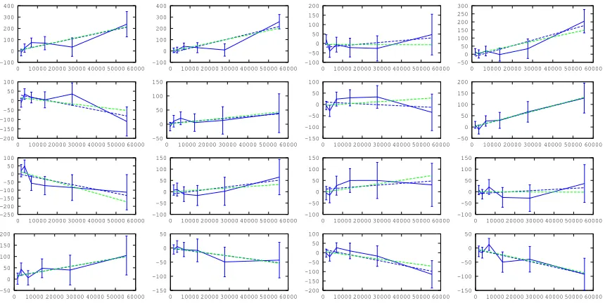
The fitted lines can be seen for the red channel of4×4example pixels in Figure 3. Even though the confidence intervals are quite large, slight variations in the pixels’ sensitivities are perceivable. At least the stronger deviations are well expressed by the linear relationship. A LS fit with uniform weighting is shown in blue for comparison.
Figure 4 visualizes the scalessc(x, y)and offsetsoc(x, y) per
pixelx, yand color channelcas images. Several patterns are noticeable, such as the out of focus dust grains in the scale image, or the vertical stripes in the offset image.
3.3 Noise reduction evaluation
-100
0 10000 20000 30000 40000 50000 60000 -100
0 10000 20000 30000 40000 50000 60000 -100
0 10000 20000 30000 40000 50000 60000 -50
0 10000 20000 30000 40000 50000 60000
-200
0 10000 20000 30000 40000 50000 60000 -50
0 50 100 150
0 10000 20000 30000 40000 50000 60000 -150
0 10000 20000 30000 40000 50000 60000 -50
0 10000 20000 30000 40000 50000 60000
-250
0 10000 20000 30000 40000 50000 60000 -100
0 10000 20000 30000 40000 50000 60000 -100
0 10000 20000 30000 40000 50000 60000 -100
0 10000 20000 30000 40000 50000 60000
-50
0 10000 20000 30000 40000 50000 60000 -150 -100 -50 0 50
0 10000 20000 30000 40000 50000 60000 -200
0 10000 20000 30000 40000 50000 60000 -150 -100 -50 0 50
0 10000 20000 30000 40000 50000 60000
Figure 3. Deviationsvl,c(x, y)−˜el,c(x, y)over˜el,c(x, y)for the red channel. Note that the 7th stop saturated the red channel and is
thus not included. Dashed lines are fitted linear FPN models (blue LS, green weighted LS of Equation 6).
Figure 4. Contrast enhanced visualization of the FPN model. Off-seto(left) and scales(right) for all three color channels.
+
Figure 5. Evaluation of the noise reduction for varying numbers of images by iteratively averaging images and computing the av-erage local variance as an estimate of the remaining noise.
of 100 images with the same camera setup as in Section 3.2, i.e. a set of 100 images that should be smooth, if not for noise. The exposure time was tweaked to achieve an image that is neither bright nor dark. The actual tone mapped sRGB color values are approximately (160 120 60). In the (16-bit) raw images, this is on average (11474.1 6148.32 2586.93).
Since the imagesshouldbe smooth in the absence of noise, the (random and fixed pattern) noise in an image can be measured by estimating the local variance in each color channel and averaging that variance over the image. The local variance vare¯c(x, y)of
an imagee¯c(x, y)is computed by replacing the usual summation
in the estimation of expected values with a Gaussian convolution that serves as a soft windowing function (Equations 10-12).
vare¯c(x, y) var(red) supressing random + fixed noise var(green) supressing random + fixed noise var(blue) supressing random + fixed noise
0 20 40 60 80 100
Figure 6. Noise reduction of the proposed approach with and without FPN for increasing numbers of images within the differ-ent color channels (denoted in corresponding color). Top: Re-maining noise variance in the 16-bit value range. Bottom: Noise reduction in dB relative to the initial noise.
E(¯ec(x, y))
As can be seen in the plots, averaging images significantly re-duces the image noise. However, even with FPN removal, the curves start to converge after about 30 to 40 images which indi-cates that the FPN model still leaves room for improvement. Of more practical significance is the observation, that for the first couple of images the gains of the FPN removal are rather small. This means that even without the, by comparison, complicated estimation of the FPN, significant gains can be achieved by just averaging a hand full of images.
3.4 Packing into 8-bit
Most SfM/MVS implementations handle images as grayscale or rgb images with 8 bits per channel. Thepeaksignal to quantiza-tion noise ratio is approximately6.02·QdB forQbits. Consid-ering this, the PSNR due to quantization noise of 48 dB is more than acceptable if the full range of 256 intensity values is used.
In the case of SfM/MVS, the matched signals are high frequency signals extracted from small patches. In the showcased “White Walls” scenario (see Section 4.1), these local image patches most definitely do not make use of the full intensity range.
In the test performed in Section 3.3, the standard deviation of the residual noise in the blue channel can be suppressed to about 29/65535 or 0.11/255 with just 20 images. By just linearly map-ping the denoised images into the 8-bit range, a substantial amount of the gained signal fidelity would be lost.
To retain these weak signals, they must be amplified, i.e. mapped to a larger interval of the 8-bit range. High frequency image structures are much more important for SfM/MVS than low quency image structures. By using a high pass filter, the low fre-quency components of the image are discarded to allow the high frequency components to make full use of the 256 value range. Since the high frequency textures are of different power in dif-ferent image regions (e.g. compare the strong texture on the seat and sofa with the weak texture on the wall in Figure 7), we use a modified Wallis filter (Wallis, 1974) which adaptively adjusts the gain based on the local variance.
As in Equation 10 let vare¯c(x, y)be the local variance ofe¯c(x, y)
and let meane¯c(x, y)be its local mean (see Equation 12). The
standard Wallis filter normalizes the signal by subtracting the lo-cal mean and dividing by the lolo-cal standard deviation. Fitting e.g. the3σrange of this normalized signal into the 8-bit value interval becomes a simple matter of scaling and shifting. Con-trary to Equations 10 and 12, however, we use a Gaussian width ofσ= 10pxfor the Wallis filter.
wc(x, y) =
$ ¯
ec(x, y)−meane¯c(x, y) p
vare¯c(x, y)
·1273 + 127.5 %
(13)
A big problem with this approach (apart from the fact that the local signal variance might be estimated as zero) is that some SfM/MVS implementations implicitly assume a constant amount of noise in the images. This can be due to reasons as simple as fixed thresholds during feature detection. However, the variance of the remaining image noise is far from constant. Firstly, the sensor noise itself is already not homoscedastic. Secondly, does the Wallis filter drastically change the amplification from image region to image region. We alleviate this problem by imposing a maximal amplification on the Wallis filter such that the3σrange of the remaining random image noise in the local neighborhood is below10/255(see Equations 14-16).
uc(x, y) =⌊(¯ec(x, y)−mean¯ec(x, y))·λc(x, y) + 127.5⌋
(14)
λc(x, y) = min
127 3·pvar¯ec(x, y)
, 10
3·pnoisec(x, y)
!
(15) noisec(x, y) = ˆnc(x, y)∗Gσ=10(x, y) (16)
The variance of the remaining random noisenˆc(x, y)is estimated
from the spread of the original imagesvi,c(x, y). These images
are, similar to Section 3.2, not all of the same brightness and if not compensated for, these fluctuations would lead to a large overes-timation of the remaining noise. We proceed as in Equation 7 by adjusting brightnesses and estimateˆnc(x, y)as in Equation 8,
albeit both with the smaller Gaussian kernel ofσ= 10px.
Note that we normalize each color channelcindividually. We also experimented with normalization based on the full local3×3
covariance matrix of the three color channels but observed no gain over the individual approach (see Figure 9). We believe that normalizing each color channel individually is sufficient to over-come quantization noise and that a full “whitening” does not add any additional benefit beyond that.
4. EXPERIMENTAL EVALUATION
A purely quantitative evaluation of the proposed noise reduction is already provided in the previous section (see Figure 6) and is based on a rather theoretical example of an image consisting completely of a homogeneous area. It was shown, that the sig-nal model incorporating truly random as well as fixed pattern noise showed the best reduction of noise within the processed images, although saturating considerably earlier than the theoret-ical bound. This section focuses on the impact of the proposed method on multi-view stereo reconstruction methods.
Two datasets have been acquired by a standard Canon EOS 400D, both containing weakly-textured areas but objects of different scales and geometry.
4.1 Wall dataset
TheWalldataset consists of images of a scene containing a couch and a chair in front of a white wall. The top of Figure 7 shows an example. Large parts of the scene are planar and visually homo-geneous areas (i.e. weakly-textured), but of different color and intensity. The scene is pictured from seven different viewpoints with30images per viewpoint and an average baseline of40cm.
In order to analyze the respective influence of the individual com-ponents, four different test cases are defined:
1. Single exposure (SE): A single JPG image is provided per viewpoint. No noise reduction or image enhancement is ap-plied (besides the camera internal processing).
2. Single exposure with Wallis filter (SEW): A single JPG im-age is provided per viewpoint. The contrast of the imim-age is enhanced by the Wallis filter.
3. Single exposure with BM3D and Wallis filter (SEBW): As 2), but the noise is locally suppressed by the BM3D filter before the Wallis filter is applied.
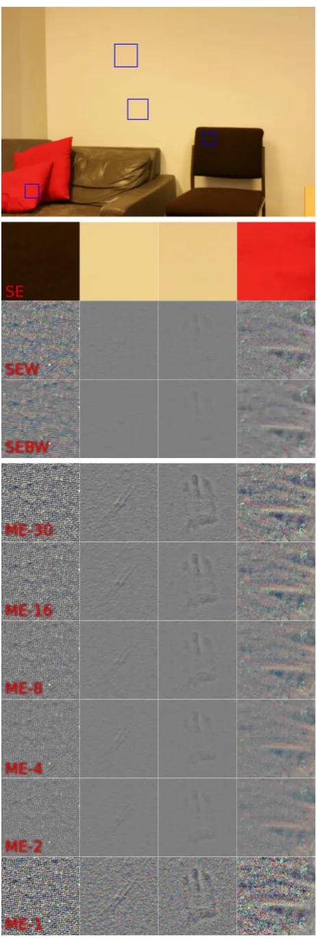
Figure 7. Noise suppression and contrast enhancement: Top: Ex-ample image (Cropped details marked in blue); From top to bot-tom: SE, SEW, SEBW, ME-30, -16, -8, -4, -2, -1crops.
The blue squares within the image shown at the top of Figure 7 denote four different image details. While the first row shows a zoom into these parts within the JPG image (SE), the second and third row show these image patches after being processed by either the Wallis filter alone (SEW) or in combination with the BM3D filter (SEBW), respectively.
The images appear grayish since the Wallis filter normalizes mean and variance of the color channels. The contrast in general and especially for fine structures is considerably increased, making small details visible that had been hidden before. The texture of the chair is clearly recognizable now, as well as small foldings of the cushion. It should be noted, that the SEW images still contain the full amount of noise, only the contrast is enhanced.
The noise in the SEBW images in the third row is locally sup-pressed by the BM3D filter before contrast is enhanced by the Wallis filter. The fine textures are mostly preserved, while the noise appears to be reduced. The image patches from the wall seem to contain image structures as well, which are not visible at all in the original SE images, but become slowly recognizable in the enhanced images (SEW as well as SEBW).
The fourth till the last row show the results of the proposed frame-work with decreasing number of images per viewpoint (ME-30, -16, -8, -4, -2, -1, respectively). Especially in the fourth row (cor-responding to ME-30) the structures on the wall become clearly recognizable: A small scratch in the wall plaster as well as a hand print. The intensity difference of these structures is so small, that they are hardly visible even for the human eye in the real world. The fewer images are used per viewpoint, the less obvi-ous the corresponding image texture is i.e. it becomes dominated by noise. The last row (ME-1) basically corresponds to the sec-ond row (SEW). The visual discrepancy is caused by a couple of subtle differences during the processing: Firstly, while the second (and third) row are based on JPG images, the proposed approach is using raw data. Thus, there are no artefacts of the JPG com-pression. Secondly, while the maximal gain had to be adjusted manually for the Wallis filter, it is automatically computed by the proposed method based on an estimate of the remaining image noise. If only a single image is used, the remaining noise is esti-mated as zero, which leads to an unconstrained gain. While the increased contrast of ME-1 is visually pleasing, it is important to note that the apparent details are mostly random noise and not actual structure. The details in ME-30 on the other hand are real, as evidenced by the plausible shading in the wall crops.
It should be noted that the visualization as discussed above is at best a qualitative cue for an increased performance. Since the application of the proposed framework is image-based 3D recon-struction, the influence on the final 3D point cloud is analyzed instead of assessing the quality of the intermediate results.
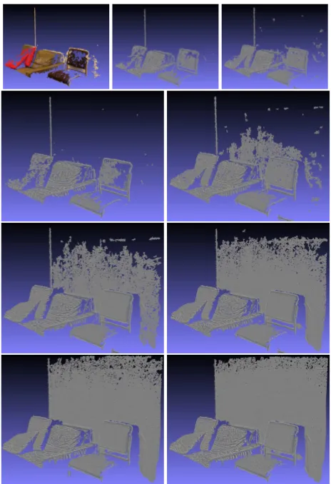
Figure 8 shows the point cloud based on the same image data as visualized in Figure 7 obtained by an successive application of the custom SfM pipeline (to obtain the camera parameters) and PMVS2 (to compute the dense reconstruction). The first row shows the reconstruction for SE (left), SEW (middle), and SEBW (right). The remaining rows show results of the proposed pipeline with increasing number of images (i.e. ME-1,-2,-4,-8,-16,-30). The number of reconstructed points is summarized in Figure 9.
Figure 8. Wall dataset. Top row: SE, SEW, SEBW; Second to fourth row: ME-1, -2, -4, -8, -16, -30images, respectively.
other parts of the scene, majorly on the backrest of the chair, are more complete.
For SEBW the changes are more prominent, visible on the right top part of Figure 8 as well as in Figure 9. Chair and cushion are significantly more completely reconstructed (the number of points increased by35%from130,939for SEW to176,782for SEBW). Interestingly, the first spots on the white wall got recon-structed as well. These points do lie on or close to the plane in contrast to the wall points reconstructed only on the basis of the unprocessed JPG images.
This indicates the importance of noise suppression for 3D recon-struction, which is even more emphasized by the results of the proposed processing chain. While the reconstruction based on a single image (ME-1) is (not surprisingly) close to the SEW point cloud, already using two images (ME-2) outperforms the SEBW-based reconstruction by far. Not only cushion as well as seat and backrest of the chair are well reconstructed, but also a sig-nificant amount of wall pixels. The number of points increased by nearly80%from132,443using one image to237,562 us-ing two images. This trend is continued by usus-ing more images per viewpoint, although the steepness of the increase becomes significantly smaller after eight images. For the maximum of 30 used images the white wall is completely reconstructed besides a few small remaining holes at the top where the cameras have less overlap. The final number of reconstructed points is591,890 -about three times as many as in the standard case of using only one unprocessed JPG image.
0 5 10 15 20 25 30
0 100000 200000 300000 400000 500000 600000
Number of images
Number of reconstructed points
SE SEW SEBW ME-N
ME-N Full-Covariance-Wallis
Figure 9. Wall dataset. Number of points of the dense reconstruc-tion for different numbers of images per viewpoint
4.2 Cat dataset
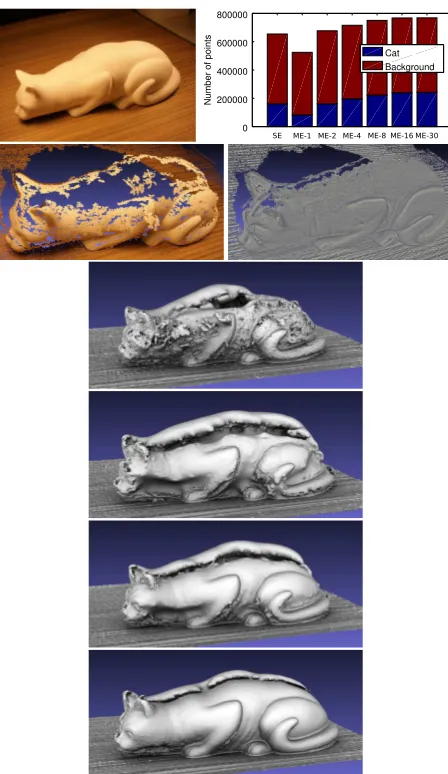
TheCatdataset consists of images of a cat sculpture. The surface is homogeneously white and shows barely any texture (in the im-ages as well as to the human eye in the real world). The top left of Figure 10 shows an example image. The dataset consists of30
images for each of the14different viewpoints with an average baseline of10cm.
Two reconstructions are conducted based on VSFM and PMVS2 using the standard data (single exposure JPG images) on the one hand as well as the proposed approach (multi exposure with mod-ified Wallis) on the other hand. The top right of Figure 10 shows the number of points within the dense reconstructions divided into two groups: Points on the cat (blue bars) and points in the background (red bars). The background (in particular the surface of the ground) contains strong texture. Consequently, both meth-ods are able to reconstruct it well and lead to a similar number of reconstructed points. Even for the cat there is not much differ-ence with respect to the number of points, if only a few images are used: The number of points increased from160,465, over
160,639, to242,250, for the standard approach and the proposed approach with2and30images, respectively. However, the accu-racy of the reconstruction differs largely. While the second row of Figure 10 shows the reconstructed point clouds of SE and ME-30, respectively, the last four rows show the meshing result based on SE, ME-1, ME-2, and ME-30, respectively. The standard ap-proach results in as many points as ME-2 (and nearly twice as many as ME-1), but roughly20%of them contain severe errors. Especially the back of the cat is either missing or reconstructed at wrong positions. The ME-1 based reconstruction (despite con-taining less points) contains less outliers. The ME-30 based re-construction is very complete as well as (visually) accurate.
5. CONCLUSION AND FUTURE WORK
Weakly-textured surfaces pose a great challenge for MVS re-constructions because the texture is effectively hidden by sensor noise and can no longer reliably be matched between images. We propose to suppress random as well as fixed pattern noise. The former through averaging of multiple exposures, the latter with the aid of a fixed pattern noise model that is estimated from test images. The enhanced image is high-pass filtered with locally varying filter gains to make better use of the limited numerical precision in 8-bit per channel images. Experiments show that the enhanced images result in significantly better reconstructions of weakly-textured regions in terms of precision and completeness.
0 200000 400000 600000 800000
Number of points
Cat Background
SE ME-1 ME-2 ME-4 ME-8 ME-16 ME-30
Figure 10. Cat dataset. Top to bottom, left to right: Example image, number of points in reconstruction, point cloud for SE, point cloud 30, mesh for SE, mesh for 1, mesh for ME-2, and mesh for ME-30.
pattern noise might as well be undesirable in some situations. The achieved gains quickly diminish after about 20 to 30 images, al-though this is already sufficient for most use-cases. Standard re-construction pipelines benefit the most of the proposed approach in cases where the texture strength is just below the threshold necessary for a successful matching.
Besides the obvious usage in MVS reconstruction, there are ad-ditional application scenarios in other areas. Light field capture is usually performed with a fixed camera rig or a slide. In this scenario repeated shooting from the same vantage point is not an inconvenience. Automatic alignment methods (such as im-plemented by Google’s HDR+ in Android) might be explored as well for applications without tripods. It is unclear though, what the impact on the internal camera calibration is. The proposed approach can easily be extended to capture wider, HDR exposure ranges by combining images of different exposure times. Initial experiments look promising, though a more thorough analysis of the benefits and use cases is necessary. Operating directly on the JPG images instead of the RAW images was tested shortly, since not all cameras allow access to the RAW image data. Although some improvements can be seen, the compression artifacts seem to be insufficiently random. It is possible that better results can be achieved if the sensor noise and thus the randomness of the artifacts is increased by selecting a higher ISO level.
ACKNOWLEDGEMENTS
This paper was supported by a grant (HE 2459/21-1) from the Deutsche Forschungsgemeinschaft (DFG).
REFERENCES
Ballabeni, A., Apollonio, F. I., Gaiani, M. and Remondino, F., 2015. Advances in image pre-processing to improve automated 3d reconstruction. In:3D-Arch - 3D Virtual Reconstruction and Visualization of Complex Architectures, pp. 315–323.
Cai, H., 2013. High dynamic range photogrammetry for light and geometry measurement. In: AEI 2013: Building Solutions for Architectural Engineering, pp. 544–553.
Dabov, K., Foi, A., Katkovnik, V. and Egiazarian, K., 2007. Im-age denoising by sparse 3d transform-domain collaborative filter-ing.IEEE Trans. Image Process16(8), pp. 2080–2095.
De Neve, S., Goossens, B., Luong, H. and Philips, W., 2009. An improved hdr image synthesis algorithm. In: Image Processing (ICIP), 16th IEEE International Conference on, pp. 1545–1548.
Debevec, P. E. and Malik, J., 1997. Recovering high dynamic range radiance maps from photographs. In: Proceedings of the 24th Annual Conference on Computer Graphics and Interactive Techniques, SIGGRAPH 97, pp. 369–378.
Furukawa, Y. and Ponce, J., 2010. Accurate, dense, and robust multi-view stereopsis.IEEE Trans. on Pattern Analysis and Ma-chine Intelligence32(8), pp. 1362–1376.
Guidi, G., Gonizzi, S. and Micoli, L. L., 2014. Image pre-processing for optimizing automated photogrammetry perfor-mances.ISPRS Annals of Photogrammetry, Remote Sensing and Spatial Information Sciencespp. 145–152.
Kontogianni, G., Stathopoulou, E., Georgopoulos, A. and Doulamis, A., 2015. Hdr imaging for feature detection on de-tailed architectural scenes. In:3D-Arch - 3D Virtual Reconstruc-tion and VisualizaReconstruc-tion of Complex Architectures, pp. 325–330.
Lehtola, V. and Ronnholm, P., 2014. Image enhancement for point feature detection in built environment. In: Systems and Informatics (ICSAI), 2nd International Conference on, pp. 774– 779.
Ley, A., 2016. Project website. http://andreas-ley.com/ projects/WhiteWalls/.
Mann, S. and Picard, R. W., 1995. On being ’undigital’ with dig-ital cameras: Extending dynamic range by combining differently exposed pictures. In:Proceedings of IST, pp. 442–448.
Ntregkaa, A., Georgopoulosa, A. and Quinterob, M., 2013. Pho-togrammetric exploitation of hdr images for cultural heritage doc-umentation. In: ISPRS Annals of the Photogrammetry, Remote Sensing and Spatial Information Sciences, pp. 209–214.
Robertson, M. A., Borman, S. and Stevenson, R. L., 1999. Dy-namic range improvement through multiple exposures. In:Proc. of the Int. Conf. on Image Processing ICIP’99, pp. 159–163.
Rothermel, M., Wenzel, K., Fritsch, D. and Haala, N., 2012. Sure: Photogrammetric surface reconstruction from imagery. In:
Proceedings LC3D Workshop, Berlin.
Wallis, K. F., 1974. Seasonal adjustment and relations be-tween variables. Journal of the American Statistical Association
69(345), pp. 18–31.
Wu, C., 2007. Siftgpu: A gpu implementation of scale in-variant feature transform (sift). http://cs.unc.edu/~ccwu/
siftgpu.
Wu, C., 2013. Towards linear-time incremental structure from motion. In: 3D Vision - 3DV 2013, 2013 International Confer-ence on, pp. 127–134.