AUTOMATIC CLASSIFICATION OF TREES FROM LASER SCANNING POINT CLOUDS
Beril Sirmacek, Roderik Lindenbergh
Department of Geoscience and Remote Sensing, Delft University of Technology, Stevinweg 1, 2628CN Delft, The Netherlands (B.Sirmacek, R.C.Lindenbergh)@tudelft.nl
Commission I/3
KEY WORDS:Point Clouds, Tree Detection, Classification, Terrestrial Laser Scanning, Mobile Laser Scanning, Airborne Laser Scanning
ABSTRACT:
Development of laser scanning technologies has promoted tree monitoring studies to a new level, as the laser scanning point clouds enable accurate 3D measurements in a fast and environmental friendly manner. In this paper, we introduce a probability matrix computation based algorithm for automatically classifying laser scanning point clouds into ’tree’ and ’non-tree’ classes. Our method uses the 3D coordinates of the laser scanning points as input and generates a new point cloud which holds a label for each point indicating if it belongs to the ’tree’ or ’non-tree’ class. To do so, a grid surface is assigned to the lowest height level of the point cloud. The grids are filled with probability values which are calculated by checking the point density above the grid. Since the tree trunk locations appear with very high values in the probability matrix, selecting the local maxima of the grid surface help to detect the tree trunks. Further points are assigned to tree trunks if they appear in the close proximity of trunks. Since heavy mathematical computations (such as point cloud organization, detailed shape 3D detection methods, graph network generation) are not required, the proposed algorithm works very fast compared to the existing methods. The tree classification results are found reliable even on point clouds of cities containing many different objects. As the most significant weakness, false detection of light poles, traffic signs and other objects close to trees cannot be prevented. Nevertheless, the experimental results on mobile and airborne laser scanning point clouds indicate the possible usage of the algorithm as an important step for tree growth observation, tree counting and similar applications. While the laser scanning point cloud is giving opportunity to classify even very small trees, accuracy of the results is reduced in the low point density areas further away than the scanning location. These advantages and disadvantages of two laser scanning point cloud sources are discussed in detail.
1 INTRODUCTION
Trees do vital job for well-being of all species on the planet. They do not only increase beauty, prove food and living space for ani-mals, but they also absorb carbon dioxide and give oxygen which contributes to the environmental circulations. Therefore, for sci-entists, for municipalities and other governmental agencies, it is important to track the numbers of trees and to measure their phys-ical attributes for scientific analysis such as carbon dioxide ab-sorbing volume. Laser scanning technology provides opportunity to do all these physical measurements in a computer environment without disturbing the nature and by spending less man effort.
Most tree classification studies in literature focus on separating trees in environments where there is little variation in objects. Therefore, separating tree points problem is solved by removing the ground points and checking the appearance of tree trunks or tree crowns. When the point cloud is from an urban region, it might contain points of many different objects such as building facades, cars, light poles, traffic signs, etc. In this case, algo-rithms need to segment the point clouds of different objects in order to control their 3D shapes. By controlling shapes, the al-gorithms decide if the points are coming from a tree or another object. These algorithms generally depend on either voxel space creation or fitting pre-defined geometrical models to the point clouds. The voxel space creation based methods are generally very sensitive to the voxel size selection. The methods which are using geometrical models also need specific parameter selection and they have a risk of missing trees which have trunk shapes different from the pre-defined models.
Some of the previously introduced approaches for processing re-gions having only trees as objects are as follows. Pyysalo and
Hyyppa (2002) introduced a method to detect individual trees in dense forest point clouds which are acquired by an airborne laser scanner. They have used a Digital Terrain Model (DTM) to remove ground, which means that additional data is required to process the point clouds. Lalonde et al. (2006b) proposed a tree classification approach from terrestrial laser scanning point clouds by detecting the ground surface. The method worked us-ing a statistical classification technique which uses linear-ness and scatter-ness of local area. The method had some disadvan-tages such as difficulty of scale selection, high computation time and difficulty of noise removal. Rutzinger et al. (2010) segmented their point cloud into homogeneous planar regions and they re-moved non-vegetation segments, which are large and planar. The remaining laser echoes are re-labelled by grouping nearby points to connected components. For these components the roughness (standard deviation of elevation) and a point density ratio in a given height interval are calculated. They observed that the point density ratio is significantly low for trees because the tree crown intercepts much more echoes than the tree trunk. Therefore, trees are extracted by selecting connected components with high rough-ness and low point density ratio.
for-Bremer et al. (2013) separated objects in the point clouds by con-nected component and Dijkstra-path analysis. They have classi-fied trees using a graph based approach considering the branch-ing levels of the given geometries. Gorte and Pfeifer (2004) have generated a range image in order to segment trees. After seg-menting individual trees, they mapped the points back to a voxel space, where it is segmented into branches using mathematical morphology. The voxel size selection has played a very crucial role in well performance of the algorithm. Tittmann et al. (2011) introduced a RANSAC approach to fit geometric models on point clouds in order to identify individual tree crowns. Li et al. (2012) introduced a method to segment individual trees in dense forest point clouds. The method depends on detecting seed points (lo-cal maximums) which are assumed as tree tops and fitting a cone shape from the seed points to the ground in order to segment the point clouds. The proposed algorithm provided good results even in dense coniferous forests. However, they have indicated that the algorithm might not be applicable to forests which consist of other types of trees. Besides, the algorithm failed to detect trees which are very short or which have low point density.
Pu et al. (2011) segmented the point cloud and checked the 3D ge-ometries of the segments. If an object has a cylindrical body and a large crown on the top, then it is labelled as a tree. The trees are not detected if their cylindrical shape trunks are not visible or if their crown diameter is not large enough. In the second case, the trees in a street point cloud might end up being labelled as poles. Monnier et al. (2012) proposed a tree detection algorithm based on local geometric descriptors computed on each laser point us-ing a fixed neighbourhood. These descriptors described the lo-cal shape of objects around every 3D laser point. A projection of these values on a 2D horizontal accumulation space followed by a combination of morphological filters helped them to detect individual tree clusters. Lalonde et al. (2006a) have extracted 3D features from the point clouds to classify points as trees and non-trees. They have then applied a segmentation algorithm to identify individuals. Finally they have used 3D primitive geomet-ric shapes such as cylinders in order to generate 3D tree models. They have used the models to estimate the breast hight diameter on ground and also aerial point clouds. Raumonen et al. (2011), proposed a method for automatically extracting approximate tree branch measures from point clouds. The method assumed that the tree can be locally approximated with cylinders without using voxel spaces. It performed well for detecting tree trunks and rel-atively large branches. However, it could not show good perfor-mance on detecting thin, irregular shaped, or low-point-density branches. Bucksch et al. (2009) detected individual trees by us-ing a region growus-ing approach startus-ing from seed points. They have used individual trees for breast height diameter estimation after skeletonizing the point clouds.
We have noticed that these graph generation, model matching and 3D feature extraction based methods not only need considerable amount of processing time, but they are also not able to detect a tree when it has a different 3D geometry than the trees which are used for training the algorithm parameters.
The literature survey shows us that; most of the previously pro-posed approaches have complex implementation steps, they
gen-ity matrix which is an imaginary surface approximately on the ground layer level. This probability matrix highlights the possi-ble tree trunk locations and it helps to identify if a point belongs to a tree. The resulting point cloud basically has the same x, y, z coordinates as the input points. However it contains one extra column which indicates if the point belongs to the ’tree’ class or ’non-tree’ class. We test the algorithm on mobile laser scanning (MLS) and airborne laser scanning (ALS) point clouds.
2 TREE CLASSIFICATION
Before identification of individual trees for further detailed anal-ysis, an important and helpful step is to classify the tree points in the input point cloud. This classification basically refers to as-signing a class value1to the points which belong to a tree and a class value0to the points which belong to other objects in the point cloud. Once tree points are separated from points sampling other objects, it is easer to identify individual trees and making necessary measurements on them.
For classifying the points in the input point cloud as tree points, we introduce a new approach based on the following steps;
1- Generating a probability matrix
2- Selecting maxima which indicate the locations having high probability to have a tree trunk
3- Assign points to the ’tree’ or the ’non-tree’ class 4- Filter the ground points
In the following parts, we explain each step in detail.
2.1 Generating A Probability Matrix
Our classification method works in 3D space and keeps the orig-inal locations of the 3D points in the cloud. However, at the processing stage, we use a 2D matrix (which we will call the V(x, y)probability matrix) for making a decision about the ap-proximate locations of the tree trunks. This 2D matrix is an imag-inary grid in the(x, y)plane, appearing between(Xmin, Ymin),
(Xmin, Ymax),(Xmax, Ymin)and(Xmax, Ymax)geographical
coordinates. Here,Xmin, XmaxandYmin, Ymaxcorrespond to
the minimum and maximum x, and y coordinate values of the input points. The grid step sizes of theV(x, y)matrix are deter-mined by considering the ground sampling resolution of the point cloud and the diameters of the smallest trees (0.5meters in our examples) that we would like to be able to classify correctly.
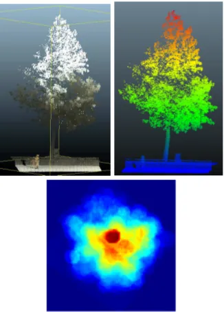
We introduce the steps of the algorithm on a tree point cloud ex-ample given in Figure 1.(a) which shows a mobile laser scanning point cloud from a view angle perpendicular to the(x, z)plane. The same point cloud is shown in Figure 1.(b) having false col-ors corresponding to the height values of the points. Figure 1.(c) shows the calculatedV(x, y)matrix which is also false colored in order to show the differences more clearly.
The pseudocode given in Figure 2 presents the algorithm that we use to compute and to assign values to the grids of theV(x, y) matrix. TheV(x, y)matrix is filled with zero values at each grid as an initial value. HerePnum is equal to the total number of
Figure 1: (a) An example tree point cloud from a mobile laser scanning data, (b) The same tree point cloud with height values assigned to the points as false color, (c) The calculatedV(x, y) matrix is shown with false colors where the red color corresponds to the highest and the blue color corresponds to the lowest value.
point cloudP respectively. TheX andY variables indicate the position of a point in the 2D grid. Finally, thexstepandystep
variables stand for the grid size inX andY dimensions respec-tively. In this study, we choosexstepequal toystep. The value
0.3(in meters) is assigned to these variables as grid step size in our example.
If the grid step size is very large then we can miss some trees which do not have a large diameter, if the step size is too small then we might use unnecessarily large memory space. Therefore, the user must decide to set the grid step size wisely considering the diameter of the smallest tree which is interesting for the ap-plication.
2.2 Selecting Local Maxima Points
The ’for’ loop in the pseudocode given in Figure 2, basically adds the height of every point into the corresponding grid. We expect theV(x, y)matrix to have very high values at the posi-tions where tree trunks are located, since there will be many trunk points which correspond to the same grids of the(x, y)plane. Therefore after generating theV(x, y)matrix, local maxima of the matrix are searched by sliding aw×wgrid size window. In our study, we choosew = 5. Since building facades, cars and other large objects do not generate local maxima in theV(x, y) matrix, we do not have a challenge to do further processing to eliminate them. However, we cannot prevent false detection of pole like objects. The detected(xt, yt)local maximums are
as-sumed as approximate tree trunk positions which unfortunately contains some light poles and traffic signs as well.
2.3 Assigning Points to Two Different Classes
The detected(xt, yt)locations are used in the classification
pro-cess that we perform with the algorithm shown in pseudocode in Figure 3.
In this pseudocode, thedistvariable is the minimum2Ddistance to the closest tree trunk position in the grid. distthresh is the
Figure 2: Pseudocode of generating the 2D probability matrix
Figure 3: Pseudocode of the algorithm for assigning tree class labels to the points
maximum allowed distance to the closest tree trunk position. So, for each 3D point the 2D Euclidean distance to the closest trunk location is determined. If this distance is below a given threshold distance then the point is assigned to that tree trunk.
2.4 Filtering the Ground Points
After assigning ”1” and ”0” labels to the points (which indicate that they are from the ’tree’ class or ’non-tree’ class respectively), we apply a filtering process in order to move some of the ground points from the ’tree’ class to the ’non-tree’ class. To do so, we use a(2∗distthresh×2∗distthresh)size window which is
located at the center of each tree trunk. Filtering is applied to the points which fall into this2Dgrid space limited by the window when they are projected on the(x, y)plane. Inside of the window, each point which has class label ”1” is checked, and the point with the lowestz position is selected as a reference (calledzl).
Again inside of the window, each point with class label ”1” is checked and the points which havezvalue lower thanzl+ztol
is moved to the ’non-tree’ class, by changing their class labels to ”0”. Here,ztol is the tolerance value that we select as10%
ofzlin our application. zlis computed again for each window
position, since it is not a global value for all input point clouds. In Figure 4, we provide the detailed mathematical steps of the ground filtering function.
cloud. As it is seen in the bottom figure, the light poles and the traffic lights are labelled as trees in the result point cloud.
Another important issue to take care of is how to choose theztol
value. If it is too high then some lower parts of the tree trunk will be eliminated. On the other hand, however, if the tree is standing on a slope or if the data is noisy (having some redundant very low values) then some of the ground points will not be filtered. In the following section, we provide results of the tree classification algorithm on mobile and airborne laser scanning point clouds.
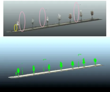
Figure 5: Top; a sub-section of the MLS point cloud having trees, light poles and traffic signs in the same row (light poles and traffic signs are shown with circles). Bottom; tree classification result of the same sub-section, which also holds the false detection of light poles and traffic signs (tree class is indicated by green color).
3 EXPERIMENTS
3.1 Data Description
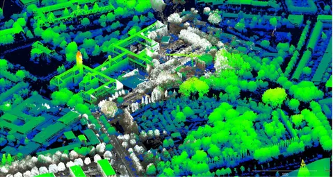
We test the algorithm on TUDelft campus point clouds which are acquired by two different sensors; one is from a mobile laser scanner and the other one is from an airborne laser scanner. The mobile laser scanning point cloud is acquired by the FUGRO company in 2013. This mobile laser scanner can collect approx-imately 11500 points per square meter with a ranging accuracy of less than 2 cm. The airborne point cloud is obtained from the free data base called ”Actueel Hooghtebestand Nederland” AHN (2008). AHN2 (the second and the higher resolution point cloud data base) data of the study region have been acquired in 2008. The AHN2 data that we use in this study is gridded in(x, y)space at 0.5 meter spatial resolution. In Figure 6, we show the original MLS and AHN2 point clouds together.
In order to evaluate the algorithm performance on different sen-sors, we take the intersecting part of the point clouds. The upper row image in Figure 8 show the intersection area of the AHN2 and MLS point clouds.
lecting tree points manually. Table 1 tabulates the performance values for AHN2 and MLS point clouds separately. The column called’Points’holds the total number of points in the input point
cloud that we process. The’Tree Points’column holds the tree
points in the groundtruth point cloud. The’Detected’column
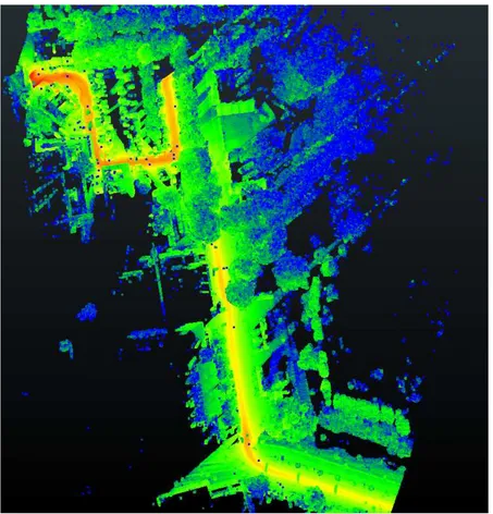
shows the true detection. However the light poles and traffic signs which are very close to the groundtruth points are also labelled as true detection. More detailed manual calculation is necessary when points coming from these non-tree objects are wanted to be eliminated. Unfortunately, the AHN2 data misses small trees since their point density does not appear high enough to be de-tected. On the other hand, the MLS data misses the trees which are further away from the road where the laser scanning vehicle has travelled. In this case, the trees which are far away from the scanning position appear in lower point densities. In Figure 7, we illustrate the point cloud density of the MLS point cloud by false coloring. The color palette assigns red for the highest and blue for the lowest local point density values. The red color points make the driving trajectory visible and it is seen that the point density decrease when the objects are further away from the laser scanning vehicle.
The last column of the table 1 shows the very low and very promis-ing computation time needed for classifypromis-ing these large point clouds. The computation time necessary for processing these two point clouds are very similar since the number of points and the surface area size are almost the same. The number of points in the input point cloud directly affects the time needed for probability matrix generation and also for assigning points to two different classes. The ground point filtering step is mostly affected by the grid size selection and the sliding window size. Smaller grid size and larger sliding window increase the computation time. The scene is also changes the computation time needed to process the point cloud. Having more trees in the scene causes having more local maxima and more distance computation in order to assign every point into the correct tree trunk.
Data Points Tree
Points
Detected %TP time (sec)
AHN2 231177 120155 111301 92,63 29,66
MLS 281405 160807 157225 97,77 29,57
Table 1: Tree classification performances on AHN2 and MLS point clouds of a large area at TUDelft campus.
3.3 Case Study
In order to present the classification performances a little bit more clearly, in Figure 9, we present the classification for a small sub-section of the MLS point cloud. We also provide Table 2 to give the exact point numbers of the clouds which are presented in the sub-figures.
Figure 6: The original AHN2 point cloud (the larger cloud) and MLS point cloud (containing the color information for each point) are shown together.
Figure 8: The intersecting AHN2 and MLS points are shown in the top and the bottom row respectively. The points which are classified as trees are shown in green.
result together with the original MLS point cloud. Finally, Figure 9(e) shows the benchmark points (in white color) and the auto-matically classified point cloud together. Here, blue points are accepted as true detection and the warmer colors are accepted as false detection since they are further away from the benchmark cloud. As can be seen in Table 2, the original MLS cloud has 524,475 points. In order to reduce the computational difficulty, this cloud is subsampled before classification. The subsampled cloud contains 21,485 points and 17,794 points are classified into the ’tree’ class automatically. By comparing the 3D Euclidean
distances to the closest benchmark points, we have concluded that 202 of 17,794 points are more than1m.further away from the benchmark. We have assumed those points as false detections. We have computed the false detection percentage in this small area as1.13%and correct detections as98.86%. As can be seen in the results given in Figure 9, the false detections are coming from the points of light poles and the cars which are parked very close to the tree trunks.
Data Points
Tree points in the original MLS section (Fig. 9(a), Fig. 9(d))
525,475
Total points in the subsampled MLS section (Fig. 9(c))
21,485
Detected tree points in the subsampled MLS sec-tion (Fig. 9(c), Fig. 9(d))
17,794
False tree detection in the subsampled MLS sec-tion (Fig. 9(d))
202
Table 2: Tree classification performances on a small section of the MLS point cloud.
4 CONCLUSIONS
This research is funded by the FP7 project IQmulus (FP7-ICT-2011-318787) a high volume fusion and analysis platform for geospatial point clouds, coverages and volumetric data set. We also give thanks to the FUGRO company in the Netherlands for providing us mobile laser scanning point clouds acquired from a part of the TUDelft campus area.
References
AHN, 2008. Actual height model of The Netherlands. http://www.ahn.nl/english.php.
Bremer, M., Wichmann, V. and Rutzinger, M., 2013. Eigenvalue and graph-based object extraction from mobile laser scanning point clouds. ISPRS Annals of Photogrammetry, Remote Sensing and Spatial Infor-mation Sciences 2(5), pp. 55–60.
Bucksch, A., Lindenbergh, R., Menenti, M. and Raman, M., 2009. Skeleton-based botanic tree diameter estimation from dense lidar data. In Proceedings of SPIE Optics and Photonics, August 2-6, San Diego, US.
Gorte, B. G. H. and Pfeifer, N., 2004. Structuring laser scanned trees using 3d mathematical morphology. ISPRS International Archives of Photogrammetry, Remote Sensing and Spatial Information Sciences 35, pp. 929–933.
Kaartinen, H., Hyypp, J., Yu, X., Vastaranta, M., Hyyppa, H., Kukko, A., Holopainen, M., Heipke, C., Hirschmugl, M., Morsdorf, F., Naesset, E., Pitkanen, J., Popescu, S., Solberg, S., Wolf, B. and Wu, J., 2012. An international comparison of individual tree detection and extraction using airborne laser scanning. Remote Sensing 4(4), pp. 950–974.
Lalonde, J., Vandapel, N. and Hebert, M., 2006a. Automatic three-dimensional point cloud processing for forest inventory. Technical Report CMU-RI-TR-06-21, Robotics Institute, Carnegie Mellon Uni-versity.
Lalonde, J., Vandapel, N., Huber, D. and Hebert, M., 2006b. Natural ter-rain classification using three-dimensional ladar data for ground robot mobility. Journal of Field Robotics 23(10), pp. 839–861.
Li, W., Guo, Q., Jakubowski, M. and Kelly, M., 2012. A new method for segmenting individual trees from the lidar point cloud. Photogram-metric Engineering and Remote Sensing 78, pp. 75–84.
McDaniel, M., Nishihata, T., Brooks, C., Salesses, P. and Iagnemma, K., 2012. Terrain classification and identification of tree stems using ground-based lidar. Journal of Field Robotics 29(6), pp. 891–910.
Monnier, F., Vallet, B. and Soheilian, B., 2012. Trees detection from laser point clouds acquired in dense urban areas by a mobile mapping system. ISPRS Annals of the Photogrammetry, Remote Sensing and Spatial Information Sciences 1(3), pp. 245–250.
Pu, S., Rutzinger, M., Vosselman, G. and Oude Elberink, S., 2011. Recog-nizing basic structures from mobile laser scanning data for road inven-tory studies. ISPRS Journal of Photogrammetry and Remote Sensing 66(6), pp. 28–39.
Pyysalo, U. and Hyyppa, H., 2002. Reconstructing tree crowns from laser scanner data for feature extraction. International Archives of Pho-togrammetry and Remote Sensing 34(3B), pp. 218–221.