PARAMETERIC ANALYSIS FOR AUTOMATED EXTRACTION OF ROAD EDGES
FROM MOBILE LASER SCANNING DATA
Pankaj Kumar a*, Paul Lewis b, Conor P. McElhinney b
a Department of Geoinformation, Universiti Teknologi Malaysia, 81310 Johor Bahru, Malaysia [email protected]
b National Centre for Geocomputation, National University of Ireland Maynooth, Ireland [email protected], [email protected]
KEY WORDS: Mobile Laser Scanning, Road Edges, Extraction, Automation, Parameters
ABSTRACT:
The applicability of Mobile Laser Scanning (MLS) systems continue to prove their worth in route corridor mapping due to the rapid, continuous and cost effective 3D data acquisition capability. LiDAR data provides a number of attributes which can be useful for extracting various road features. Road edge is a fundamental feature and its accurate knowledge increases the reliability and precision of extracting other road features. We developed an automated algorithm for extracting left and right edges from MLS data. The algorithm involved several input parameters which are required to be analysed in order to find their optimal values. In this paper, we present a detailed analysis of the dimension parameters of input data and raster cell in our algorithm. These parameters were analysed based on temporal, completeness and accuracy performance of our algorithm for their different sets of values. This analysis provided the estimation of an optimal values of parameters which were used to automate the process of extracting road edges from MLS data.
* Corresponding author
1. INTRODUCTION
An accurate 3D information about the location of terrestrial objects along with their geometrical and structural properties supports a wide range of services and evidence based decision making. Geospatial information contributes to the production of useful knowledge which can be used to develop more efficient approaches for managing urban infrastructures and natural resources (Coote and Smart, 2010). Laser scanning systems enable the acquisition of an accurately georeferenced set of dense 3D LiDAR point cloud data. Other benefit of this system is the high level of automation and the ability of this system to acquire data beneath tree's canopy. The information obtained through laser scanning systems have applications in road safety, urban planning, flood plain, glacier and avalanche mapping, bathymetry, geomorphology, forest survey, bridge and transmission line detection.
The use of laser scanners onboard terrestrial based moving vehicles has led to the collection of high quality 3D data. The applicability of these Mobile Laser Scanning (MLS) systems has increased for the mapping of route corridor and its surrounding environment due to the rapid, continuous and cost effective data acquisition capability (Barber et al., 2008; Haala et al., 2008). LiDAR data provides a number of attributes including elevation, intensity, pulse width, range and multiple echo information, which can be used for extracting features. It is a rich source of 3D georeferenced information whose volume and scale have inhibited the development of automated algorithms. The large volume of data produced by modern-day MLS systems lead to time-consuming and computational expensive process for automated feature extraction (Kumar, 2012). For example, Riegl VQ-250 mobile laser scanner generates 300,000 points per second resulting in approximately 20GB of data per hour.
An accurate knowledge about road edges increases the reliability and precision of road features extraction. Road edges are needed to be correctly identified and extracted in order to estimate road geometry and physical road objects along the route corridor. In Kumar et al. (2013), we presented an algorithm for extracting left and right edges from MLS data. The developed algorithm was based on a novel combination of two modified versions of the parametric active contour or snake model. The algorithm involved several input parameters which are required to be analysed in order to use their optimal values in the algorithm. This paper deals with a detailed investigation of the dimension parameters of input data and raster cell in our road edge extraction algorithm. The use of their optimal values in the algorithm provides us to automate the process of extracting road edges. In Section 2, we present a review of various automated methods which have been developed for extracting road and its boundaries from LiDAR point cloud data. In Section 3, we provide a brief overview of our road edge extraction algorithm as presented in Kumar et al. (2013). In Section 4, we present a detailed analysis of input parameters that provides us to understand the importance of using their optimal values in the algorithm. We discuss the output results in Section 5 and finally, conclude our paper in Section 6.
2. LITERATURE REVIEW
features. Several methods have been developed over the past decade for extracting road and its boundaries from LiDAR data.
Hu et al. (2004) developed an automated road extraction approach in which LiDAR data was segmented based on elevation and intensity attributes. The Hough transformation and morphological operations were then applied to extract the candidate road stripes and open parking areas. High resolution image was also used to obtain candidate areas by extracting the concrete or asphalt pixels based on thresholding. Accuracy issues associated with the intermixing of road networks with parking areas were resolved using shape analysis and vehicle detection queues from the LiDAR and image data. Akel et al. (2005) identified roads from airborne LiDAR data which were used for generalising the Digital Terrain Model (DTM). LiDAR data was segmented by applying a region growing approach on the basis of surface normal direction and height difference properties and then the extracted segments were classified into road and non-road objects based on a certain set of decision rules. Yuan et al. (2008) proposed an algorithm for extracting road surface from terrestrial LiDAR data. The algorithm used a fuzzy clustering method to cluster LiDAR points that belong to a scan line. Straight lines were fitted to the linearly clustered data using slope information for extracting the road surface area. Tseng et al. (2007) developed an approach for surface reconstruction from terrestrial LiDAR data. In their approach, a surface was grown from an initial seed point in the LiDAR data based on the extended snake model. The internal energy was provided by placing a constraint on the angle in between the normal vectors of two adjacent planar patches while the external energy was modelled as a function of distance from the LiDAR points to the corresponding planar patch. Samadzadegan et al. (2009) presented an automated approach to extract road from airborne LiDAR data based on classifier fusion method. Multiple classifier system was used to classify the LiDAR points into road and non-road objects using first pulse, last pulse, range and intensity attributes. Different combinations of LiDAR attribute layers were classified based on different features using maximum likelihood and minimum distance methods. McElhinney et al. (2010) developed an automated algorithm to extract road edges from MLS data. A set of lines were fitted to the road cross-sections based on the navigation data and then LiDAR points within the vicinity of the lines were determined. The estimated points were analysed based on slope, intensity, pulse width and proximity to vehicle information in order to extract the road edges. Serna and Marcotegui (2013) presented an automated approach for analysing urban accessibility using MLS data. In their approach, LiDAR range attribute based interpolated image was segmented using λ-zones algorithm and curb candidates were selected using height and elongation criteria. Finally, close curbs were reconnected using Bezier curve and then obstacle map was prepared to analyse the accessibility for wheelchair users.
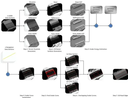
Most of the automated road extraction methods are based on delineating roads by distinguishing them from non-road objects but do not make attempt to extract the road edges. The developed approaches do not provide any detailed analyses of their input parameters which are required to automate the process of road extraction. A detailed investigation of these parameters is required in order to use their optimal values in the algorithm. In the next section, we provide a brief overview of parametric model, the snake is represented as a controlled spline curve, which is implemented based on computed energy (Kass et al., 1988). It is defined within a 2D image domain that moves towards a desired object boundary under the influence of an internal energy within the curve itself and an external energy derived from the image data. A workflow of the road edge extraction algorithm is shown in Figure 1.
In our algorithm, we input n number of l m × w m × h m LiDAR and n number of l m navigation data sections, where l, w and h refers to length, width and height. The dimensions of input data sections are selected based on analysis as presented in Section 4. We select the input data sections with an overlap of 2m between them which allows us to batch process consecutive and overlapped road sections as required in the algorithm. We use the LiDAR elevation, reflectance and pulse width attributes in the algorithm which are converted into 2D raster surfaces to reduce computational expense. In Step 1 of our algorithm, multi resolution terrain pyramids are generated from the LiDAR attributes and then 2D raster surfaces are estimated from the first level terrain pyramids using natural neighbourhood interpolation in Step 2 (Crawford, 2009; ESRI, 2010). The cell size, c parameter required to generate the raster surfaces is selected based on experimental analysis as provided in Section 4. Slope values are estimated from the elevation stiffness properties with an empirically estimated values of α and weight parameters. The step size of snake curve is pulse width raster surfaces respectively through the consecutive use of hierarchical thresholding and Canny edge detection. In the hierarchical thresholding approach, the mask size, Mslope, Mref, Mpw and threshold, Tslope, Tref, Tpw parameters are applied to the slope, reflectance and pulse width raster surfaces respectively (Sonka et al., 2008). The mask size is used to blur the raster surface with a Gaussian convolution kernel and is determined based on the level of noise. A larger mask size is used when there is a high amount of noise present in the raster surface, while a small mask size is used when there is little or no noise. The threshold parameter can be estimated using the difference between the brightness value of an object cell and representative background cells in the raster surface. The hierarchical thresholding approach outputs raster surfaces with only two values, 255 for object cells and 0 for non-object cells. We input these surfaces into the Canny edge detection in which upper threshold, T1 and lower threshold, T2 parameters are applied (Canny, 1986). The values of mask size and threshold parameters are empirically estimated while the values of upper and lower threshold parameters are set as 250 and 5 respectively, based on the output cell values obtained from the hierarchical thresholding. The balloon external energy is included by providing a weight to the normal unit vector of the
snake points. Thus, GVF external energy terms attract the snake curve while balloon external energy helps push it outwards towards the object boundaries. The weight parameters for the balloon (κ1) and GVF (κ2, κ3, κ4) energy terms are selected empirically after examining their several combinations and are fixed for all the road sections.
In Step 4, the snake curve is initialised over a 2D raster surface based on the navigation track of mobile van along the road section. We initialise the snake curve in the form of parametric ellipse using ϕ and ω angle parameters. The ϕ angle is calculated from the average heading angle of the mobile van along the road section under investigation while the ω angle is selected empirically and fixed for the road sections with similar width. In Step 5, the snake curve moves under the influence of internal and external energy terms. It approaches the minimum energy state and converges to the road edges during an iterative process. In Step 6, we obtain overlapping snake curves by batch processing consecutive individual road sections. The intersection points in between the overlapping snake curve points are found and then non-road edge points in between the intersection points are removed. This results in one continuous snake with the left and right edges for the complete road section. Finally in Step 7, the third dimension is provided to the extracted left and right road edge points by finding the elevation value from the nearest LiDAR point to each road edge point. In the next section, we provide a detailed analysis for estimating optimal dimensions of input data and raster cell in our algorithm.
4. AUTOMATION ANALYSIS
The automation of our road edge extraction algorithm required a detailed analysis of the input parameters. In the following sections, we present the analysis of two parameters.
4.1 Input Data Dimensions
We performed this analysis to find the optimal dimensions of the data section to which our road edge extraction algorithm can be applied. The dimensions of input data sections were optimally estimated as they impact the process efficiency in terms of computational cost. The selection of 30m width ensured the inclusion of road in the data while 5m height was useful in order to remove the impact of vertical objects such as trees, road signs, light poles along the route corridor on the raster surface interpolation. To find the optimal length with respect to computational efficiency, we considered three test cases in which a temporal performance of our road edge extraction algorithm was analysed in a road section with 10m, 20m and 30m length. We selected one national primary road section consisting of grass-soil edges with shoulders. To process this road section, we used three 30m × 10m × 5m, 30m × 20m × 5m, 30m × 30m × 5m sections of LiDAR data and three 10m, 20m, 30m sections of navigation data. The processed data was acquired using the eXperimental Platform (XP-1) MLS system which has been designed and developed at National University of Ireland Maynooth (NUIM) (Kumar et al., 2014, 2015).
Figure 1: Road edge extraction algorithm (Kumar et al., 2013)
In each test case, we applied our road edge extraction algorithm to the road section using a cell size c=0.06m2, Mslope=185, Mref=25, Mpw=25, Tslope=45, Tref=132, Tpw=55, T1=250, T2=5,
α=9, =0.001, =3, κ1=1, κ2=4, κ3=2, κ4=2 and ϕ=-37.270. The value of ϕ was calculated from the average heading of the mobile van along the selected road section. The number of iterations were selected empirically for which the snake curve was able to successfully converge to the road edges. The number of GVF iterations used were 600 while the number of iterations required to move the snake curve were 40. The variation in road length required slight modification of two parameters in the algorithm, as shown in Table 1.
Road Length (m)
Ω (degree)
δt (radian)
10 340 0.03
20 170 0.015
30 110 0.01
Table 1: Different parameters used in the three test cases of input data dimensions analysis.
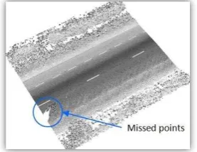
We applied the higher Mslope parameter to the slope raster surface due to inherent noise. This noise was due to missing points in the section of LiDAR data, shown in Figure 2, which are due to the mobile van overtaking a stationary vehicle during the data acquisition process along the road section. In the reflectance and pulse width raster surfaces, the use of a lower,
Mref and Mpw, parameters respectively was sufficient to remove the inherent noise. The values of Ω and δt were decreased proportionally to reflect the change in the length of the road section. The final positions of the snake curve in the three test cases are shown in Figure 3.
4.2 Raster Cell Dimension
A suitable cell dimension is required in order to calculate a 2D raster surface. The selection of the optimal cell dimension is essential as it may affect the accuracy and computational cost of our road edge extraction algorithm. To find its optimal value, we analysed the performance of our road edge extraction
algorithm in raster surfaces generated with different cell dimensions. We selected one 10m section of rural road consisting of grass-soil edges. To process this road section, we used one 30m × 10m × 5m section of LiDAR data and one 10m section of navigation data which was collected with the XP-1 MLS system.
We considered six test cases in which raster surfaces were generated with cell dimensions 0.02m2, 0.04m2, 0.06m2, 0.08m2, 0.1m2 and 0.2m2 from the LiDAR elevation, reflectance and pulse width attributes. These dimensions were selected with decreasing and increasing values based on an average point spacing of 0.08m in the LiDAR points. In each test case, we applied our road edge extraction algorithm to the road section with the following parameters: Mslope=25, Mref=25, Mpw=25, T1=250, T2=5, α=9, =0.001, κ1=1, κ2=4, κ3=2, κ4=2, ω=200 and
ϕ=21.490. These parameters were found empirically after examining several values in the algorithm. The ϕ value was calculated from the average heading angle of the mobile van along the selected road section. The number of iterations required to converge the snake curve to the road edges was 40. Some of the parameters used in the algorithm were different in each case to correctly test the effect of cell dimensions, as shown in Table 2.
Cell Size (m2)
Tslope Tref Tpw δt GVF Iteration
0.02 75 100 85 1 0.01 1800 0.04 60 100 70 2 0.02 900
0.06 55 100 65 3 0.03 600 0.08 50 100 65 4 0.04 450 0.1 40 100 65 5 0.05 360
0.2 30 100 65 10 0.1 180
Table 2: Different parameters used in the six test cases of raster cell dimension analysis.
We used different sets of T, the hierarchical threshold parameter in each case. The value of was increased to decrease the snake curve step size during one iteration, δt was increased to decrease the number of points in the snake curve, while the number of GVF iterations were decreased. These parameters were changed to account for the effect of the change the raster surfaces resolution would have on the algorithm. The , δt and GVF iteration parameters were changed proportionally to the change in the cell size of the raster surfaces. The final positions of the snake curve in the six test cases are shown in 4. In the next section, we analyse the output results and discuss them. Figure 2: Missed points as circled in blue in the section of
LiDAR data.
Figure 3: Final position of the snake curve over the slope raster surface with (a) 10m, (b) 20m and (c) 30m road length.
Figure 4: Final position of the snake curve over the slope raster surface with (a) 0.02 m2, (b) 0.04 m2, (c) 0.06 m2, (d) 0.08 m2,
(e) 0.1m2 and (f) 0.2m2 cell dimension.
5. RESULTS & DISCUSSION
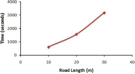
We examined the results obtained in both the analyses for estimating optimal dimensions of input data and raster cell in the algorithm. In all cases of input data analysis, the snake curve was able to converge to the road edges. We estimated the time take by the snake curve to move from its initial position to the final position in the three test cases as shown in Figure 5. In the first case, the snake curve required around 623 seconds to move
to the final position. In the second and third case, the snake curve was computationally expensive as it required 1570 and 3191 seconds respectively to converge to the road edges. This analysis was performed on a computer with 2 Intel Xeon E5607 processors @2.27 GHz, 12GB RAM and a 64-bit operating system. For example, to process a 60m section of road with 30m × 10m × 5m would require approximately 3738 seconds, with 30m × 20m × 5m would require 4710 seconds and with 30m × 30m × 5m would require 6382 seconds, without overlap. Thus, on the basis of computational cost, we chose the 10m length of the road section to which our road edge extraction algorithm can be applied.
In the raster cell dimension analysis, we also estimated the time taken by the snake curve to move from its initial position to the final position for each test case. A plot of these estimates is shown in Figure 6. For cell sizes 0.02m2 and 0.04m2, the snake
curve required more time with 5280 and 1327 seconds respectively, to converge to the road edges. The increased time taken was due to the use of higher resolution raster surfaces. With cell sizes of 0.06m2 and 0.08m2, the snake curve required
moderate time with 384 and 178 seconds respectively, to move to the final position. In the final two cases, the snake curve required less time with 78 and 9 seconds respectively. This reduced time was due to the use of lower resolution raster surfaces.
We estimated the length of both the left and right road edges as extracted in each test case of the raster cell dimension analysis. In each case, a plot of completeness was obtained from the snake curve as determined from the left and right edges, as shown in Figure 7. For cell dimensions 0.02m2, 0.04m2, 0.06m2
and 0.08m2, the snake curve converged to more than 79% of the left and right road edges. In the 0.1m2 cell dimension case, the snake curve converged to around 75% of the left road edge and 72% of the right road edge while in the large cell dimension of 0.2m2, the snake curve converged to around 55% of the left road edge and 45% of right edge. In our road edge extraction algorithm, the road edges are extracted using iterative partially overlapping road sections. The 0.1m2 and 0.2m2 cell cases produced snake curves which were not able to converge to the road edges to the extent with which the overlapping snake curves can be obtained.
The left and right edges extracted in each test case were validated based on their comparison with manually digitised road edges. We manually digitised the left and right edges in the road section from the 3D LiDAR data. The digitisation can introduce an absolute error in the manual process of selecting the road edge points in a 3D environment. However, they were utilised in the validation approach to perform relative accuracy analysis of the road edges extracted in each test case. We estimated the 3D Euclidean distance between the extracted and digitised road edge points at a 0.5m interval. The statistical analysis of the estimated distance values was carried out for the left and right edges as shown in Tables 3 and 4 respectively. The negative and positive values for the left and right edge
0.02 0.04 0.06 0.08 0.1 0.2
min -0.087 -0.071 -0.106 -0.134 -0.073 -0.121
max 0.108 0.097 0.078 0.056 0.044 0.175
mean 0.008 0.011 -0.011 -0.019 0.001 0.024 median 0.005 0.026 0.011 -0.014 0.01 0.021
Table 3: Statistical analysis for the left edges in the six test cases of raster cell dimension analysis.
points respectively indicate that the extracted edges were outside the digitised edges of the road surface. Similarly, the positive and negative values for the left and right edge points respectively indicate that the extracted edges were inside. Based Figure 5: Plot of the time taken by the snake curve to move
from its initial position to the final position in the three test cases of input data dimension analysis.
Figure 6: Plot of the time taken by the snake curve to move from its initial position to the final position in the six test cases of
raster cell dimension analysis.
Figure 7: Plot of completeness obtained from the snake curve in the six test cases of raster cell dimension analysis.
on the minimum and maximum values, the highest accuracy for the left edge was obtained by applying the 0.1m2 cell dimension while for the right edge using the 0.02m2 cell dimension. A mean and median value close to 0 indicates high accuracy. For the left edge, the cell dimensions whose mean and median Table 4: Statistical analysis for the right edges in the six test
cases of raster cell dimension analysis.
For the 0.02m2 and 0.04m2 cell dimensions, the snake curve was computationally expensive without providing any considerable improvement in the accuracy of the extracted road edges. In the 0.1m2 and 0.2m2 cell dimension cases, the snake curve took less time to move to the final position, however it did not converged to the road edges to the extent that will allow for overlapping snake curves to be obtained. Overlapping snake curves are required to process multiple road sections and to facilitate general application of the algorithm. For the 0.06m2 cell dimension, the minimum-maximum range, mean and median accuracy values were better than in the 0.08m2 cell dimension. The snake curve in the 0.06m2 case required a reasonable amount of time to move from its initial position to the final position and was able to converge to the road edges to the extent with which the overlapped snake curves can be obtained. Thus, we chose an optimal cell dimension of 0.06m2 to generate the raster surfaces from the LiDAR attributes. In the next section, we conclude our paper.
6. CONCLUSION
Our automated road edge extraction algorithm is based on the combination of GVF and balloon parametric active contour models. In Kumar et al. (2013), we tested our algorithm on different types of road sections representing rural, urban and national primary road sections. The successful extraction of these road edges from the multiple distinct road sections validates our algorithm. The algorithm involved several input parameters which are required to be thoroughly investigated. We presented a detailed analysis of the dimension parameters of input data and raster cell in the algorithm. These parameters were analysed on the basis of temporal, completeness and accuracy performance of our algorithm for their different set of values. The selection of their optimal values is essential as it may affect the accuracy and computation cost of our road edge extraction algorithm. The internal and external energy weight parameters were selected empirically, however, they are required to be analysed experimentally in order to find their robustness in the algorithm. In the raster cell dimension analysis, the extracted road edges were validated based on their comparison with manually digitised road edges. In this validation approach, we manually estimated the Euclidean distance between the extracted and digitised road edge points at certain interval. There is a need to develop an automated and efficient approach for qualitative validation of the extracted road edges. The algorithm is also required to be tested on large
and complex road sections in order to demonstrate its robustness for extracting road edges.
ACKNOWLEDGEMENTS
The research presented in this paper was initially funded by the Irish Research Council (IRC) Enterprise Partnership Scheme and Strategic Research Cluster grant 07/SRC/I1168 of Science Foundation Ireland (SFI). The research was continued at Universiti Teknologi Malaysia (UTM). The authors gratefully acknowledge this support.
REFERENCES
Akel, N. A., Kremeike, K., Filin, S., Sester, M. and Doytsher, Y., 2005. Dense DTM generalization aided by roads extracted from LiDAR data. In: The International Archives of Photogrammetry, Remote Sensing and Spatial Information Sciences, Enschede, The Netherlands, Vol. 36(3/W19), pp. 54– 59.
Barber, D., Mills, J. and Smithvoysey, S., 2008. Geometric validation of a ground-based mobile laser scanning system. ISPRS Journal of Photogrammetry and Remote Sensing, 63(1), pp. 128–141.
Canny, J., 1986. A computational approach to edge detection. IEEE Transactions on Pattern Analysis and Machine Intelligence, 8(6), pp. 679–698.
Coote, A. and Smart, A., 2010. The value of geospatial information to local public service delivery in England and Wales. Available at: www.lga.gov.uk/GIresearch (11 June, 2015).
Crawford, C., 2009. Minimizing noise from LiDAR for contouring and slope analysis. Available at: http://blogs.esri.com/esri/arcgis/2009/09/02 (28 December, LiDAR mapping for 3D point cloud collection in urban areas - a performance test. In: The International Archives of Photogrammetry, Remote Sensing and Spatial Information Sciences, Beijing, China, Vol. 36(B5), pp. 1119–1124.
Hu, X., Tao, C. V. and Hu, Y., 2004. Automatic road extraction from dense urban area by integrated processing of high resolution imagery and lidar data. In: The International Archives of Photogrammetry, Remote Sensing and Spatial Information, Istanbul, Turkey, 35(B3), pp. 320–324.
Kass, M., Witkin, A. and Terzopoulos, D., 1988. Snakes: Active Contour Models. International Journal of Computer Vision, 1(4), pp. 321–331.
Kumar, P., 2012. Road features extraction using terrestrial mobile laser scanning system. Ph.D. Dissertation, National University of Ireland Maynooth p. 300.
Kumar, P., Lewis, P., McElhinney, C. P. and Rahman, A. A., 2015. An algorithm for automated estimation of road roughness from mobile laser scanning data. The Photogrammetric Record, 30(149), pp. 30–45.
Kumar, P., McElhinney, C. P., Lewis, P. and McCarthy, T., 2013. An automated algorithm for extracting road edges from terrestrial mobile LiDAR data. ISPRS Journal of Photogrammetry and Remote Sensing, 85, pp. 44–55.
Kumar, P., McElhinney, C. P., Lewis, P. and McCarthy, T., 2014. Automated road markings extraction from mobile laser scanning data. International Journal of Applied Earth Observation and Geoinformation, 32, pp. 125–137.
McElhinney, C. P., Kumar, P., Cahalane, C. and McCarthy, T., 2010. Initial results from european road safety inspection (EURSI) mobile mapping project. In: The International Archives of Photogrammetry, Remote Sensing and Spatial Information Sciences, Newcastle, UK, Vol. 36(5), pp. 440–445.
Samadzadegan, F., Bigdeli, B. and Hahn, M., 2009. Automatic road extraction from LIDAR data based on classifier fusion in urban area. In: The International Archives of Photogrammetry, Remote Sensing and Spatial Information Sciences, Paris, France, 38(3/W8), pp. 81–86.
Serna, A. and Marcotegui, B., 2013. Urban accessibility diagnosis from mobile laser scannning data. ISPRS Journal of Photogrammetry and Remote Sensing, 84, pp. 23–32.
Smadja, L., Ninot, J. and Gavrilovic, T., 2010. Road extraction and environment interpretation from LiDAR sensors. In: The International Archives of Photogrammetry, Remote Sensing and Spatial Information Sciences, Saint-Mande, France, 38(3A), pp. 281–286.
Sonka, M., Hlavac, V. and Boyle, R., 2008. Image processing, analysis and machine vision. Second edition, Thomson Engineering, New York.
Tseng, Y. H., Tang, K. P. and Chou, F. C., 2007. Surface reconstruction from LiDAR data with extended snake theory. Energy Minimization Methods in Computer Vision and Pattern Recognition (EMMCVPR) pp. 479–492.
Xu, C. and Prince, J. L., 1997. Gradient vector flow: a new external force for snakes. In: Proceedings of Computer Vision Pattern Recognition, San Juan, US, pp. 66–71.
Yuan, X., Zhao, C. X., Cai, Y. F., Zhang, H. and Chen, D. B., 2008. Road-surface abstraction using ladar sensing. In: Proceedings of 10th International Conference on Control, Automation, Robotics and Vision, Hanoi, Vietnam, pp. 1097-1102.