ACCURACY ASSESSMENT OF GO PRO HERO 3 (BLACK) CAMERA IN
UNDERWATER ENVIRONMENT
Helmholz, P.*, Long, J., Munsie, T., Belton, D.
Department of Spatial Sciences, Curtin University, GPO Box U 1987, Perth WA 6845, Australia (Petra.Helmholz, John.Long, D.Belton)@curtin.edu.au, [email protected]
Commission V, WG V/3
KEY WORDS: Calibration, underwater, action camera, lens distortion, quality assessment
ABSTRACT:
Modern digital cameras are increasing in quality whilst decreasing in size. In the last decade, a number of waterproof consumer digital cameras (action cameras) have become available, which often cost less than $500. A possible application of such action cameras is in the field of Underwater Photogrammetry. Especially with respect to the fact that with the change of the medium to below water can in turn counteract the distortions present. The goal of this paper is to investigate the suitability of such action cameras for underwater photogrammetric applications focusing on the stability of the camera and the accuracy of the derived coordinates for possible photogrammetric applications. For this paper a series of image sequences was capture in a water tank. A calibration frame was placed in the water tank allowing the calibration of the camera and the validation of the measurements using check points. The accuracy assessment covered three test sets operating three GoPro sports cameras of the same model (Hero 3 black). The test set included the handling of the camera in a controlled manner where the camera was only dunked into the water tank using 7MP and 12MP resolution and a rough handling where the camera was shaken as well as being removed from the waterproof case using 12MP resolution. The tests showed that the camera stability was given with a maximum standard deviation of the camera constant σc of 0.0031mm for 7MB (for an average c of 2.720mm) and 0.0072 mm for 12MB (for an average c of 3.642mm). The residual test of the check points gave for the 7MB test series the largest rms value with only 0.450mm and the largest maximal residual of only 2.5 mm. For the 12MB test series the maximum rms value is 0. 653mm.
* Corresponding author
1. INTRODUTION
The use of Photogrammetry is no longer limited to a small group of experts. It is increasingly used by a number of disciplines and therefore becoming more pronounced in the modern spatial sciences community. The two main factors contributing to the development are new emerging camera technologies as well as affordable and user friendly software. Modern digital cameras are increasing in quality whilst decreasing in size. For instance, in the last decade, a number of waterproof consumer digital cameras (action cameras) became available, often costing less than $500. A popular model of action cameras is the GoPro and it may be a viable option for future projects having adequate resolution and quality in both image and video, matching that of far larger digital SLR cameras.
Many of those cameras use fisheye lenses which are often not suitable for geometric accurate photogrammetric applications – at least for above water applications. Previous studies (Balletti, et al., 2014) have concluded that the wide field of view of sports cameras, intensified by the convex lens adopted by sports cameras distort the imagery considerably. However, with the change of shooting medium to below water, the medium can in turn counteract the distortion, therefore being appropriate for underwater photogrammetry (Shortis, 2015).
Furthermore, Photogrammetry allows for the observation of precise and accurate measurements and is non-destructive. Therefore, it is an attractive technology for a number of disciplines such as marine ecology. Possible applications include the monitoring of marine fauna populations (Shortis and
Harvey, 1998) and the estimation of fish sizes (Harvey et al., 2003; Costa et al., 2006; Trobbiani et al., 2015). Other possible underwater photogrammetric applications includes structural analysis of sub-sea structures (Dare and Fraser, 2000), ocean mapping (Bodenmann et al., 2010), mapping and detailing of historical shipwrecks (Hollick et al., 2013) and inspection of coral reef structures (Burns et al., 2015).
Expense is a key factor in surveying, especially underwater. Producing the highest quality results for the lowest amount of money is important when pursing an economic solution for every problem. Underwater photogrammetry is relatively expensive in the field of spatial sciences with initial start-up cost of cameras and funding of expedition to location, with necessary crew and supplies. Only a handful of specialised teams operate in the field of underwater photogrammetry. Introduction of cost effective, high definition compact cameras in the last 5 years with underwater capability as discussed created a new option in the field of underwater photogrammetry. Off the shelf availability and ease of use further adds to the appeal. Introducing a low cost option with the perceived notion that these compact underwater cameras will be suitable for photogrammetry means an increase in users and practical applications. Current photogrammetry practices may be able to substitute the digital action cameras for current camera setups and methods if it can be demonstrated that this type of camera is proven in terms of stability, consistency and accuracy. Therefore, the objective of this paper is to investigate these aspects of an action camera, specifically in regards to the Go Pro Hero 3 (black) series. For this purpose multiple GoPro sports cameras have been employed to test the consistency and
stability of the interior orientation parameters as well as the accuracy of derived coordinates.
The paper is outlined as follow: After related work is presented in the next section, the data capturing and processing are introduced. These sections are followed by the calibration results and the accuracy analysis. The paper closes with a conclusion and outlook.
2. RELATED WORK
In the last few years, action cameras are becoming more and more popular for photogrammetric applications, however the use of small format cameras for photogrammetric applications is not novel and a number of papers have been published dealing with their stability (e.g. Mitishita et al., 2010). The main reasons for the popularity is that they are easy to handle, that they are able to provide still and video images, and that that they are capable to perform under extreme conditions (Belletti et al., 2014). These reasons and that they are quite light and relatively inexpensive make them especially attractive for underwater and UAV applications. However, a careful calibration is essential (because of effects such as strong fisheye distortions). After a successful calibration, action cameras show potential for being used for photogrammetric applications (e.g. Belletti et al., 2014).
In this paper we will especially focus on the usability of action cameras for Underwater Photogrammetry. The use of Photogrammetry to observe precise and accurate measurements underwater is not novel and has been used in the past for a number of applications such as the non-destructive monitoring of marine fauna populations (Shortis and Harvey, 1998) and the estimation of fish sizes (Harvey et al., 2003; Costa et al., 2006; Trobbiani et al., 2015). These underwater applications’ overall goal is usually the reliable determination of length measurements. For instance, in the field of marine ecology the accuracy of the length measurement of fish is particular critical when they are used to estimate the fish biomass, as errors are magnified during the calculations (Harvey et al., 2002). The reliability of these results depends on the quality of the calibration and the stability of the system.
When operating underwater the refractive index of water is different compared to the index above water. This leads to significant differences in the calibration parameters. In addition, the refraction index in water is known to change with depth, temperature and salinity (Shortis, 2015). However, in the underwater environment, not only the effects of refraction need to be corrected or modelled, but also the entire light path including the camera lens, housing port and water medium (Shortis, 2015). The primary effect of the refraction through the air-port and port-water interfaces will be radially symmetric around the principle point and are accounted for in the radial lens distortion parameters (Shortis, 2015). In contrast, alignment errors between the optical axis and the housing port and possible non-uniformities in the thickness or material of the housing will lead to asymmetric effects which will show in the de-centric calibration parameters (Shortis, 2015). Furthermore, the shape of the camera housing and port may change with depth due the changing pressure (Shortis and Harvey, 1998). The most significant sensitivity for the calibration stability of underwater is the relationship between the camera lens and the housing (Shortis, 2015). Rigid mounting of the camera in the housing is critical to ensure that the total optical path from the image sensor to the water medium is consistent (Harvey et al., 1998). Telem and Filin (2012) even suggested adding additional
calibration parameters which account for the multimedia effect and the inaccuracy related to the setting of the camera in the housing. To conclude, a calibration of the system should always be performed and if possible in-situ (or in really similar conditions) as all of the above mentioned factors will lead to a change of the camera calibration parameters. planar test fields have two main weaknesses. Firstly, it increases the risk of undesirable correlations between the calibration parameters, and secondly, the network is externally constrained and therefore does not allow the updating from the network solution (self-calibration). Using two Sony HDR-CX700 HD camcorders mounted on a rigid base bar Boutros et al. (2015) showed that using a 3D calibration field leads to a significantly better result in improving the precession and accuracy of the measurements. When using two or more cameras, the arrangement of the cameras also influences the achievable precision and accuracy (Harvey et al., 2010; Boutros et al., 2015) as well as the resolution of the used camera system (Harvey et al., 2010).
Shortis and Harvey (1998) assessed the stability of their introduced a stereo video system in regards to its precision and accuracy. The video system consisted of two Sony Hi8 video cameras in water tight cases convergent (8 degrees) mounted on a frame with a distance between them of 1.4m, achieving a base to distance ratio of 3.8. The self-calibration was performed using a 3D calibration field on 16 synchronised pairs of frames; the locations of the targets are measured manually. The expected object space precision of 3mm and 22mm (95% confidence level) in lateral position and depth could be achieved when testing the system on 16 plastic silhouettes of fish ranging in size from 100 to 490mm in length, and placed at a distance between 2.5 and 6.6 m away from the cameras with multiple measurements. The mean precision across all silhouettes were ±4mm with a range of ±2mm to ±13mm and only showed weak correlation with the length and orientation of the silhouettes. The mean accuracy across all silhouettes was -12.7mm with a range of ±3.7mm to ±-25.3mm and again only showed weak correlation with the length and orientation of the silhouettes.
Capra et al., (2015) investigated three different low cost digital cameras for the accuracies of metric underwater photogrammetry applications; Canon Power Shot G12 (a regular low cost digital camera) and two sports cameras, the Intova Sport HD and the GoPro HERO 2. A calibration frame was used at sea with a depth of roughly 15m for an in-situ calibration using Agisoft PhotoScan. The maximum detected total error was 0.524mm for the Canon PowerShot G12 camera, 43.037mm for the GoPro Hero and 11.330mm for the Intova Sport HD. It was concluded that the SFM algorithm implemented by the camera calibration software PhotoScan could not correctly handle the relative distortion caused by the action cameras. Nevertheless, the paper gives an estimation of the accuracy of low cost digital camera in metric Underwater Photogrammetry.
In this publication we will perform the calibration of three GoPro Hero 3 (Black) action cameras in a number of different set outs. A 3D dimension target field divided in Ground Control Points (GCPs) and Check Points will be used for the calibration
and accuracy evaluation. The aim is to investigate into the interior orientation consistency by comparing multiple iterations from the cameras applying different resolutions and conditions. The values will be compared amongst the same camera and then contrasting against the other cameras.
3. DATA CAPTURING AND PROCESSING 3.1 Camera
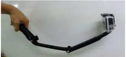
All equipment was planned and compiled prior to testing. The cameras are all the same make and model; light compact sports cameras from the GoPro Hero 3+ Black series, the highest quality GoPro available at the time of testing. Each camera is identical and in good working condition. For the testing the cameras were mounted on a GoPro Extender Handle (Figure 1).
Figure 1: GoPro mounted on GoPro Extender Handle.
GoPro cameras have a small fixed focal length, with the camera having a reasonable large f/2.8 aperture (GoPro, 2015) in relation to the lens size. Therefore, subjects of GoPro images will be in focus from a close range (centimetres) to infinity. A description of aspects of the GoPro is shown in Table 1. The serial numbers of the used cameras are #305E917, #3064F7C, and #3064F72. In the paper, there are respectively referred to as “GB”, “GD” and “GT”.
Image sensor C-MOS, 1/ 2.5” Max. resolution (Pixels) 4000 x 3000 Max. resolution (MP) 12
Lens aperture f/2.8
FOV (underwater) 92 degrees
Pixel size 0.00155 mm
Dimension 59 x 41 x 30mm
Weight with housing 136 grams Table 1: Specification GoPro 3 (Black).
3.2 Data capturing
Due to the nature of this investigation a large body of water in a controlled environment was required to submerge and capture images of the calibration frame. The water must be clear enough for the frame to be visible at 1-2 meters away and also be still enough as to not disrupt the position during data capturing. Curtin’s Centre for Marine Sciences and Technology (CMST) water tank was used for testing. The tank is 3 meters long, 2 meters wide and 1.5 meters in depth with water filling the tank enough to submerge the calibration frame fully. In the centre of the tank a 3D calibration frame was placed. A sufficient amount of light projecting into the testing tank was present to illuminate calibration features whilst submerged. Enough room about the tanked allows easy manoeuvrability of the camera around the frame. Figure 2 shows the test tank with submerged calibration frame.
Figure 2: Controlled test field environment - calibration frame in water tank.
Image capturing was completed in 2-3 sessions. The GoPro camera was submerged with the extender arm, rotating it around the calibration frame whilst maintaining a constant distance. 120 degrees surrounding the frame being optimal and could be achieved (125 ± 10 degrees). Multiple images of the calibration frame were taken for each calibration sequence. Some images suffered from motion blur and were excluded from the analysis. However, as more than the minimum number of required still images was captured, eight to ten sharp images were available per sequence. One camera position was tilted by 90 degrees per sequence. All settings of the cameras were kept fixed in all sequences.
For calculation of the interior orientation parameters and accuracy assessment test a 3D calibration frame was used. The calibration frame has 52 reference marks along two planes. These series of targets must be stable as during the capturing, otherwise it could adversely affect the results. Each mark has a spatial location in an arbitrary coordinate system in millimetres. The marks have been set systematically placing multiple along the same axis, giving a good spread for capturing. While 25 marks are used as Ground Control Points (GCP), 27 marks are used as Check Points (CP). All marks are observed in as many images as possible; the number of measurements range between two and ten times per mark. The GCPs were chosen evenly across the bottom and top of the calibration frame for an even spread.
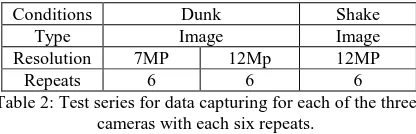
The camera stability is expected to vary due to handling, pressure change and movement stresses on the camera frame and housing, as well as the possibility of the cameras moving within the housing. While minimal changes are expected as long as the camera is not removed from the waterproof case, i.e. only “dunk(ed)” into the water tank, higher deformations are expected when the camera is removed from the waterproof case, the memory card and the battery are removed, and the camera handled in a rough manner, i.e. “shake”. The raw handling and shaking of the camera simulates the stress normally forced on the camera during transportation. Therefore, the following tests as summarise in Table 2 were performed for each camera. Three cameras (GT, GB, GD) were tested in three different test series (7MP dunk, 12MB dunk, 12MP shake) with each 6 repeats leads to 54 sampling sequences. Each sequence contains at least 8 images with 52 reference mark to be observed in each image, i.e. a minimum of 432 observations were made per sequence,
leading to a total number of over 23k observations in all
Table 2: Test series for data capturing for each of the three cameras with each six repeats.
A target centroiding feature was used to centre reference marks on the calibration frame for camera calibration, enabling a high precision when referencing.
3.3 Data processing
A bundle adjustment with self-calibration is performed in order to determine the parameter of the interior orientation, i.e. the calibrated focal length (c), the position of the principle point in the image plane (xP, yP), the parameter of the radial distortion (k1, k2, k3) and de-centric distortion (p1, p2). The used software for observations and adjustment is iWitnessPro; a review of calibration procedures and algorithm is available in Luhman et al. (2015). Also computed are the residuals of Ground Control and Check Points. All pass and check points are observed manually.
4. RESULTS
The three cameras are assessed under different aspects. Firstly, interior orientation consistency will be assessed (test 1). During this test the values of the interior orientation parameters will not only be compared amongst the same camera, but also in contrast to the other cameras. Next, the derived residuals of the Check Points will be used to evaluate the accuracy of the cameras using different resolution levels and handlings.
4.1 Test 1 – Stability of the interior orientation parameters The results from the first calibration test including the average indicating a high precession. The camera constant parameter is similar for each camera with an average 2.730mm and a Table 3: Interior Orientation parameters of all three cameras
using the 7MB dunk test series (in mm).
Table 4 summarised the calibration parameters similar to Table 3 but uses the 12MB dunk images instead of the 7MB dunk images. The average camera constant is 3.644mm with a
standard deviation of 0.00094mm between the cameras. That the camera constant and also all other parameters are significant different from the previous table was as expected as changing the resolution basically equates to another camera being used. However, similar to the last table all parameters are similar. The standard deviations are also in general small with only some exceptions. The exceptions are highlighted in the table and are all regarding the radial and de-centric distortion parameters. The reason for the increased values is suspected to be a systematic influence which will be discussed later.
GB GD GT Table 4: Interior Orientation parameters of all three cameras
using the 12MB dunk test series (in mm).
Finally Table 5 shows the calibration results of the 12MB shake test. The camera calibration values between the cameras are again quite consistent between the different cameras, showing again only slight inconsistencies for the radial and de-centric distortion parameters as highlighted in Table 5. The average camera constant is 3.640 mm with a standard deviation of 0.0077. These numbers are also quite coherent with the results presented in Table 4 (12MB dunk). Therefore, we can say that Table 5: Interior Orientation parameters of all three cameras
using the 12MB shake test series (in mm).
By analysing all of the highlighted values in Table 3 to Table 5 no single sequence could be identified for being the reason for the high standard deviations. In all cases two or three sequences contributed to the high value.
4.2 Test 2 – Accuracy Assessment
From the calibration process, a bundle adjustment is performed and the coordinates of check points are observed. A summary of the results including the average residual (res), root mean square (rms) and maximal absolute residual value (max|res|) for the 7MB dunk test is shown in Table 6. While the average residuals as well as the rms values look fine, the maximal res indicating some errors (highlighted values in Table 6). Indeed looking at the res and rms values of each single sequence, one faulty sequence could be discovered within the six taken sequence of each camera for the 7MB dunk test. Similar faulty
sequences were also visible in the 12MB dunk test (for all cameras) and the 12 MB shake test (only for the GB camera). The observed errors could also be verified with the residual plots.
GB GD GT
value value value
res x -1.03 3.05 0.24 0.04 0.89 1.50 res y 1.49 3.12 0.17 0.11 -0.32 1.26 res z 0.89 0.34 0.78 0.24 0.53 0.28
rms x 2.97 0.24 1.63
rms y 3.22 0.20 1.19
rms z 0.94 0.81 0.59
max|x| 18.73 275 9.84
max|y| 18.58 85.25 8.38
max|z| 18.66 495 7.33
Table 6: Average residual (res), root mean square (rms) and maximal absolute residual value (max|v|) of all check points in
mm (7MB dunk).
After removing the sequences which were detected to contain an error, the results for the 7MB dunk test could be achieved for the res, rms and max|res| results, as shown in Table 7. All res values are small; most of the rms values are around to 1mm and the maximum res values indicating just some smaller blunders. Interesting is that the res, as well as the rms and max values for z are often much higher than the equivalent x and y values are. This can be expected for a normal photogrammetric accuracy assessment because of the geometry.
GB GD GT
res x 0.2181 0.2481 0.2755
res y 0.2114 0.1553 0.1883
res z 0.7835 0.7761 0.6294
rms x 0.9423 0.9676 0.9016
rms y 0.9978 1.0103 0.9238
rms z 1.2336 1.2740 1.0430
max|x| 2.5071 2.5437 2.5241
max|y| 3.0832 2.9930 2.8101
max|z| 5.9287 5.0363 4.4537
Table 7: Average residual (res), root mean square (rms) and maximal absolute residual value (max|v|) of all check points in
mm (7MB dunk) after removing the sequences containing errors.
12 MB dunk 12 MB shake
GB GD GT GB GD GT
res x 0.260 0.185 0.232 0.254 0.260 0.179 res y 0.203 0.105 0.193 0.269 0.272 0.224 res z 0.855 0.065 0.405 1.085 0.637 0.499 rms x 1.026 0.977 0.855 1.027 0.945 0.870 rms y 1.113 0.962 0.888 1.227 0.991 0.939 rms z 1.464 1.176 0.997 1.834 1.041 0.956 max|x| 2.984 4.570 2.899 3.984 3.759 2.488 max|y| 3.101 2.847 3.058 3.281 2.775 2.527 max|z| 5.801 12.329 4.204 6.522 4.384 4.690 Table 8: Average residual (res), root mean square (rms) and maximal absolute residual value (max|v|) of all check points in
mm (12MB dunk and shake) after removing the sequences containing errors.
Table 8 summarized the res, rms and max|res| results of the 12 MB dunk and shake tests. Similar to Table 7 the res and rms values are really small and indicating a good accuracy of the three cameras which are also comparable to each other.
However, the maximal residual value of again especially the z values indicating a systematic trend.
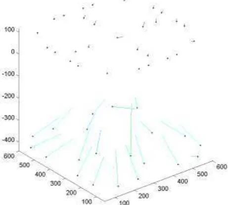
A systematic trend is easily visible in the residual plots. A representative plot is given in Figure 3; the z-direction is pointing to the camera i.e. the top plane is closest to the camera position. It is important to point out that this trend is not only visible within one camera or one test series but through all sequences, with only the magnitudes of the trends varying slightly. This indicates a systematic error coming from the calibration frame.
Figure 3: Representative 3D residual plot (here: 12MB dunk GT, test 5). Units are in mm with an enhancement factor for the
residuals of 50.
As the goal of this paper is to show the accuracy and the precision of the camera and not of the calibration frame this systematic trend was removed. This was achieved by calculating the average of the residuals within each test series (e.g. 7MP dunk GB, 7MP dunk GD, 7MB dunk GT…) and then to calculate the residuals from this average position. If the test series was the same, then variation between coordinates should be small. The results for three the 7MP dunk series are shown in Table 9. All residuals are small; the largest rms value is only 0.450mm. The largest maximal residual is only 2.521mm.
GB GD GT
res x 4.0E-07 -4.0E-07 2.0E-07
res y 4.0E-07 4.0E-07 4.0E-07
res z 4.0E-07 -2.0E-07 4.0E-07
rms x 0.1119 0.171 0.1527
rms y 0.1299 0.190 0.1128
rms z 0.3103 0.450 0.2605
max|x| 0.7603 1.7928 0.6955
max|y| 0.7096 1.4589 1.1488
max|z| 1.7068 2.5209 2.1284
Table 9: Average residual (res), root mean square (rms) and maximal absolute residual value (max|v|) of all check points in mm (7MB dunk) after removing the sequences containing errors
and after removing the systematic trend.
Similar good are the results for the 12MB dunk and 12MB shake series. The maximum rms value is 0.653mm and the largest maximum residual is 3.781mm again in the z direction.
12 MB dunk 12 MB shake
GB GD GT GB GD GT
res x 4E-07 -2E-02 4E-07 -0.036 3E-07 -3E-07 res y -2E-07 5E-04 4E-07 -0.004 3E-07 3E-07 res z 2E-07 -4E-02 -2E-07 0.139 -3E-07 3E-07 rms x 0.244 0.428 0.405 0.247 0.196 0.253 rms y 0.188 0.353 0.328 0.187 0.154 0.282 rms z 0.517 0.587 0.653 0.490 0.356 0.391 max|x| 1.437 2.742 1.611 1.424 1.517 1.426 max|y| 0.741 1.508 1.566 1.282 1.091 1.558 max|z| 2.766 3.781 2.684 2.087 2.176 2.050 Table 10: Average residual (res), root mean square (rms) and maximal absolute residual value (max|x|) of all check points in
mm (12MB dunk and shake) after removing the sequences containing errors and after removing the systematic trend.
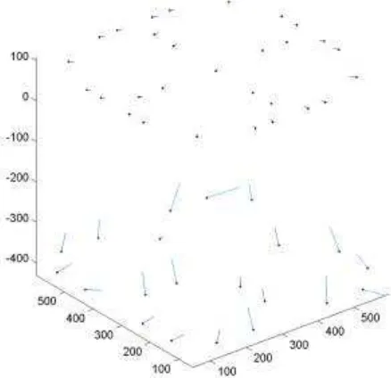
Figure 4 shows the residual plot of the same test as in Figure 3 after the systematic trend was removed. The residuals are much smaller and show a more random pattern. However, the figure shows that the residuals in the further plane are systematically larger than those observed on the closest plane.
Figure 4: Representative 3D residual plot (here: 12MB dunk GT, test 5) with removed systematic trend. Units are in mm with
an enhancement factor for the residuals of 50.
A pattern of large residuals on the bottom of the calibration can also be explained due to impeded view of the rear of the frame, leading to less intersecting between reference marks producing lower accuracy. Some of these check points were reference as little as 2-5 times due the angle at which the images were taken. Vice-versa the reference marks at the top of the frame can be seen and reference from all images such that these marks will contain less error.
5. CONCLUSION AND OUTLOOK
In this paper we could shown that the consistency of the interior orientation parameters are stable and validated using multiple GoPro cameras in different test sets. The same GoPro cameras in the same environment using the same resolutions are able to remain stable in its interior orientation despite the abuse. We also could show that the removal of the camera from the waterproof body and rough handling during the experiments did not influence the camera calibration parameters significantly.
Mitishita, et al. (2013) determined for a small format digital camera (Kodak DCS Pro 14n - similar to the GoPro cameras) for above water testing a standard deviation of the camera constant σc of 0.012mm. The maximum σc for our 7MB tests was 0.0031 mm and for our 12MB was 0.0072 mm, hence achieving significant better results as Mitishita, et al. (2013). However, as Mitishita, et al. (2013) concluded that his value was precise and sufficient enough to not cause significant effect on the measuring ability, this can be also conclude for the GoPro cameras for underwater applications.
When analysing the precision and accuracy of the GoPro cameras using 27 check points of a calibration frame we were able to detect a deformation in the calibration frame which is to be suspected around 3mm in the z-direction. For our 7MB test series the largest rms value was only 0.450mm and the largest maximal residual only 2.5 mm. For the 12MB test series the maximum rms value is 0. 653mm and the largest maximum residual is 3.781mm. The large maximum residual of 3.781mm indicating remaining blunders and can also be explained due to impeded view of the rear of the frame, leading to less intersecting between reference marks. The results indicate that GoPro camera can achieve accuracy suitable for close range Underwater Photogrammetry applications as long as correct photogrammetric workflow is followed. This means an in-situ calibration using a 3D calibration frame with check points and repeating the measurements at least three times.
The results should be verified with a “re-calibrated” calibration frame. The goal of future research includes to not only capture still images but also video sequences and to analyse the extracted frames of these video sequences.
The future direction of underwater photogrammetry is not defined; however, photogrammetry is transitioning into the adoption of off the shelf digitals cameras as they improve. If these ‘action’ digital cameras are correctly calibrated to a high quality they are sufficient in terms of metric reconstruction of physical objects as their accuracy can reach a sufficient level to be acceptable for purposes of underwater surveys.
ACKNOWLEDGEMENTS
Curtin’s Centre for Marine Science and Technology (CMST) to provide with the calibration frame and the kindly use of their water tank facility.
REFERENCES
Boutros, N., Shortis, M., Harvey, E., 2015. A comparison of calibration methods and system configurations of underwater stereo-video systems for applications in marine ecology. Limmology and Oceangraphy: Methods, vol. 13, pp. 224-236.
Balletti, C., Guerra, F., Tsioukas, V., Vernier, P., 2014. Calibration of actin cameras for photogrammetric purposes. Sensors. Vol. 14, pp. 17471-17490.
Bodenmann, A., Thornton, B., Ura, T., Sangekar, M., 2010. Pixel mapping for generation of 3D coloured seafloor bathymetry using a single camera. Autonomous Underwater Vehicles (AUV), 2010 IEEE/OES, pp. 1-9.
Bruno, F., Bianco, G., Muzzupappa, M., Barone, S., Razionale, A., 2011. Experimentation of structured light and stereo vision for underwater 3D reconstruction. ISPRS Journal of Photogrammetry and Remote Sensing, Vol. 66, pp. 508-518.
Burns, J. H. R., Delparte, D., Gates, R. D., Takabayashi, M., 2015. Utilizing underwater three-dimensional modelling to enhance ecological and biological studies of Coral reefs. Int. Arch. Photogramm. Remote Sens. Spatial Inf. Sci., XL-5/W5, 61-66, 2015
Capra, A., Dubbini, M., Bertacchini, E., Castagnetti, C., Mancini, F., 2015. 3D Reconstruction of an underwater archaeological site: comparison between low cost cameras. The International Archives of the Photogrammetry, Remote Sensing and Spatial Information Sciences, XL-5/W5, pp. 67-72, ISPRS Underwater 3D Recording and Modelling Workshop 2015.
Costa, C., Loy, A., Cataudella, S., Davis, D., Scardi, M., 2006. Extracting fish size using dual underwater cameras. Aquaculture Engineering, Vol. 35, pp. 218-227.
Dare, P. M., Fraser, C. S., 2000. Linear infrastructure mapping using airborne video imagery and subsequent integration into a GIS. Geoscience and Remote Sensing Symposium, 2000. Proceedings. IGARSS 2000, IEEE 2000 Vol.5, pp. 2299 – 2301.
Harvey, E., Shortis, M., 1998. Calibration stability of an underwater stereo-video system: Implications for measurement accuracy and precision. Marine Technology Society Journal, Vol. 32, pp. 3-17.
Harvey, E., Fletcher, D., Shortis, M., 2002. Estimation of reef fish length by divers and by stereo-video: A first comparison of the accuracy and precision in the field on living fish under operational conditions. Fisheries Research, Vol. 57, No. 3, pp. 255-265.
Harvey, E., Cappo, M., Shortis, M., Robson, S., Buchanan, J., Speare, P., 2003. The accuracy and precision of underwater measurements of length and maximum body depth of southern Bluefin tuna (Thunnus maccoyii) with a stereo-video camera system. Fisheries Research. Vol. 63, pp. 315-326.
Harvey, E., Goetze, J., McLaren, B., Langlois, T., 2010. Influence of range, angle of view, image resolution and image compression on underwater stereo-video measurements: High-Definition and Broadcast-Resolution Video Cameras Compared. Marine Technology Society Journal, Vol. 22, No. 1, pp. 75-85.
Hollick, J. Belton, D., Moncrieff, S., Woods, A., Hutchison, A., Helmholz, P., 2013. Creation of 3D models from large unstructured image and video datasets. The International Archives of the Photogrammetry, Remote Sensing and Spatial Information Sciences, XL-1/W1, pp. 133-137, ISPRS Hannover Workshop 2013.
Luhmann, T., Fraser, C., Maas, G.-H., 2015. Sensor modelling and camera calibration for close-range photogrammetry. ISPRS Journal of Photogrammetry and Remote Sensing, http://dx.doi.org/10.1016/j.isprs.2015.10.2006.
Mitishita, E., Cortes, J., Centeno, J., Machado, A., Martins, M., 2010. Study of stability analysis of the interori orientation parameters from small-format digital camera using on-the-job calibration. Int. Arch. Photogramm. Remote Sens. Spatial Inf. Sci, XXXVIII part 1, on CD.
Shortis, M., Harvey, E.S., 1998. Design and calibration of an underwater stereo-video system for the monitoring of marine
fauna populations. The International Archives of the Photogrammetry, Remote Sensing and Spatial Information Sciences, Vol. XXII, pp. 792-799.
Shortis, M., 2015. Calibration techniques for accurate measurements by underwater camera systems. Sensors. Vol. 15, pp. 30810-30827.
Telem, G. and Filin, S., 2010. Photogrammetric modelling of underwater environments. ISPRS Journal of Photogrammetry and Remote Sensing, Vol. 65, pp. 433-444.
Trobbiani, G. and Venerus, L., 2015. A novel method to obtain accurate length estimates of carnivorous reef fishes from a single video camera. Neotropical Ichthyology, Vol., 13(1), pp. 93-102.