International Review of Economics and Finance 8 (1999) 343–362
Noise trading, transaction costs, and the
relationship of stock returns and trading volume
Charles Kramer*
International Monetary Fund, Room 9-612, 700 19th St. NW, Washington, DC, 20431, USA
Received 13 May 1997; accepted 21 January 1998
Abstract
This article constructs an economic model of a rational trader who operates in a market with transaction costs and noise trading. The level of trading affects the rational trader’s marginal cost of transacting; as a result, trading volume (through its effect on marginal cost) is a source of risk. This engenders an equilibrium relationship between returns and volume. The model also provides a simple way to scrutinize this relationship empirically. Empirical evidence supports the implications of the model. 1999 Elsevier Science Inc. All rights reserved.
JEL classification:G12; G14
Keywords:Capital asset pricing model (CAPM); Noise trading; Trading volume
1. Introduction
The last few years have seen a resurgence of interest in the empirical relationship between stock prices and trading volume. Recent studies find significant statistical relationships between volume and returns, in terms of the level of returns, its volatility and its autocorrelation. Other studies explore intertemporal causality and feedback
between returns and volume.1The linkages between theory and empirics are rarely
explored in a way that is most useful for applied researchers, however. I propose a model that links trading volume to equilibrium returns in a simple, intuitive way, in the context of a standard equilibrium model. Both direct and indirect evidence supports the model.
* Corresponding author. Tel.: 202-623-8491; fax: 202-623-6339.
E-mail address: [email protected] (C. Kramer)
Recent results raise a variety of questions about financial markets. Finance research-ers and practitionresearch-ers might wonder whether a relationship of returns and volume is at odds with equilibrium models such as the Capital Asset Pricing Model (CAPM). Regulators might be interested in the implications for market efficiency. For example, transactions taxes are sometimes proposed as a mechanism for reducing the effects of speculation on asset prices.2Regulators would like to know whether such measures
will work, and what side effects they might cause. One is unable to answer these questions from a purely empirical approach, of course; the analytical tools of financial economics must be applied.
These findings are confusing when analyzed from an economic perspective, though. If price reflects fundamental value, it is hard to say why rational agents should care about trading volume at all. Some authors motivate the relation of volume to returns by arguing that fundamentals traders act as market makers for liquidity traders, or that irrational traders have persistently biased expectations.3 Others examine the
microstructure of asset markets with asymmetric information.4 It is difficult to link
these models to classical theories of asset pricing, however, as they typically use a highly stylized environment and one or two assets. These features also limit the degree to which they can be implemented empirically.
One feature of markets that may engender a relationship between returns and volume is transaction costs. Suppose demand for risky shares by noise or liquidity traders evolves at random. For example, following Delong et al. (1990a), some investors may form their opinions randomly; or, following Campbell, Grossman, and Wang (1993), their risk aversion may fluctuate randomly, leading to perturbation in their optimal portfolio. Suppose also that the market has a fundamentals trader, who trades securities for the usual motive of hedging intertemporal shifts in marginal utility. This fundamental trader must pay transaction costs to trade shares. If the volume of noise trading influences the marginal cost of transacting, it can also influence equilibrium prices. Thus, a relationship of price and volume may exist that is consistent with rational pricing, albeit rational pricing that takes noise trading into account as a risk factor (through its influence on marginal costs). Moreover, there are already some arguments that transaction costs may figure in the relationship between returns and volume.5In principle, this relationship could go either way: quiet markets could imply
high transaction costs (through an absence of liquidity and high spreads) or low ones (if markets are quiet due to the absence of noise trading, there may be lower costs of gathering information because trades are more informative).6
2. Model
The model is based on the Lucas (1978) model of intertemporal choice. An infinitely-lived representative agent is assumed to characterize the aggregate choices of a hetero-geneous group. Assets are sources of real income, denominated in terms of a single, nonstorable consumption good. At each date, the agent plans future consumption and investment to maximize the expected discounted value of future utilities.
When the representative agent goes to the market to trade, he competes with noise traders. Such traders may buy and sell shares based on rumors, speculation, or bad investment advice; they may also trade to manage liquidity.7The rational agent takes
the actions of such traders into account, as the volume of trade influences the marginal cost of transaction.
This idea makes sense at a practical level. It is well-known among finance prac-titioners that market depth influences the cost of transaction. For example, the bid-asked spread is a function of the inventory cost of the market maker, which in turn relates to the level of activity in the market.8 More frequent trading implies lower
carrying and order-processing costs per share for the market maker. On the other hand, if high trading volume reflects a preponderance of well-informed traders, the market maker’s adverse-selection costs will be high, and so must be the bid-asked spread. Market depth is also an important consideration in determining which assets to hold in a managed fund, and the optimal frequency of trading.9
The necessary notation is as follows:vt(K31) denotes the current period’s amount
of noise trading in K assets. I do not model the decision process of noise traders explicitly, but merely treat noise trading as a random process that is not controlled by the rational decision maker.10 The rational agent knows v
tat timet, but not vt11.
This makes sense, as real-world traders can observe current market activity as they trade.11 However, this does not mean that noise trading is irrelevant. Noise trading
risk affects decisions now, because those decisions take uncertainty about the future into account. Uncertainty about the future includes uncertainty about future noise trading, and hence future transaction costs and consumption.
I also do not model the trading process, the evolution of the supply of shares, or the equilibration of supply and demand for securities. These are not necessary given the setup of the model. One might picture, however, all agents trading through market makers who hold inventory. In this case asset demands by rational and noise traders are unlinked; demand by noise traders need not equal total supply less demand by rational traders. This also implies that noise traders’ demands are inelastic with respect to transaction costs; otherwise the level of fundamentals trading could influence noise trading.
mean that the optimization problem is well-posed. Of course, in some theory models, the role of noise traders is considerably different, and modeled in more detail. How-ever, the simplicity of this model affords access to many standard tools, including empirical ones, which one could not use otherwise.
For the rational side,U(•) denotes a one-period utility function, assumed concave, bounded, and twice differentiable.ctdenotes period-tconsumption of the single good.
b e(0,1) denotes an impatience parameter, used to discount future utilities.xt(Kx1)
denotes the number of shares of the claim to output held by the rational agent at datet. yt(1xK) denotes this period’s output, distributed to shareholders as dividends.
ptdenotes the (1xK) vector of share prices (in consumption units). Dxt ;xt 2xt21
denotes the (Kx1) vector of changes in the number of shares held by the rational agent between periods t21 and t.
f(|Dxt|; vt), f:RkxRk . R1is a transaction-costs function, twice differentiable,
qua-siconvex and increasing inxt, withf(0vt) 50.12f(•) is meant to capture all the costs
of trading to the agent that vary with trading, including brokerage fees. While the bid-asked spread is not modeled explicitly, it can be though of heuristically as one
component. With this notation, the agent’s optimization problem for date t can be
written as follows [Eq. (1)]:
subject to the sequence of budget constraints [Eq. (2)]:
ct1ptxt1 f(|Dxt|;v) #(yt1pt)xt21 (2)
where Et denotes conditional expectation. Because the budget space is convex and
the program is discounted, the standard sufficient conditions for a unique equilibrium pricing functionp(y) to exist are satisfied.13
The first-order conditions for optimal investment xt, assuming an interior
maxi-mum, is
2U9(ct)(pt1ft9) 1EtbU9(ct11)(yt11 1 pt11 1f9t11) 501xK (3)
wheref9t (1xK) denotes the gradient of f(•;•) with respect to xt(given xt21and vt).
Eq. (3) is the usual Euler equation of optimality with an adjustment for transaction costs. As usual, the representative agent chooses the best portfolio when the marginal cost of giving up one unit of consumption this period just counterbalances the marginal expected return from investing the unit and consuming it next period. The only difference from the usual case is that these marginal quantities include the cost of investing the unit of consumption this period and cashing it in next period.
3. Implications for equilibrium returns
The Euler Eq. (3) can be manipulated in standard ways to yield implications for equilibrium returns.14 For example, rearrangement of Eq. (3) shows thatE
t(Rit11) is
U9(Ct). The expressionE(Mt11ft11/pt) is identical to the Brock (1982) expression for
the Ross (1976) Arbitrage Pricing Theory (APT) risk premium, where the systematic risk factor is transaction cost as a fraction of price (ft11/pt). Hence, marginal cost is
a priced risk factor; because marginal cost is a transformation of trading volume, trading volume (here, aggregate trading volume) also behaves like a priced risk factor. This fact has both time-series and cross-sectional implications. In time-series, well-known features of trading volume (seasonality, for example) that are manifested in time-variation in the covariation between marginal utility and transaction costs could give rise to similar time-series behavior in expected returns. In the cross-section, if f(•) differs across assets, there will be concomitant implications for the cross-sectional distribution of returns. Consider two assets that are identical except for trading costs. Suppose that the first has zero trading costs and the second has trading costs that are a nondegenerate function of trading volume. The second asset will have a positive premium for the risk associated with transactions costs, and hence have a higher expected return than the first. Similar conclusions would follow from assuming that the argument offi(•) is the trading volume for stockI, rather than aggregate trading
volume, and that the first asset has very high trading volume (so thatf91(•) is negligible)
and that the second asset has very low trading volume (so thatf92(•) is large).
The Euler equation can also be used to derive a consumption CAPM in the presence of transaction costs when there are many assets. Denote byRc
it5(Pi,t111Yi,t111
fi,t11)/(Pi,t 1fi,t) the rate of return net of transaction costs. Suppose there exist a risk
free or ‘zero-beta’ asset and a reference or market portfolio, with cost-adjusted returns denoted Rand Rrespectively. Then, manipulation of Eq. (3) yields
Et[Rci,t11] 2 Rcf,t115 gi,t{Et[Rcm,t11] 2Rcf,t11}
where
Yi,t ;
Covt(Mt11,Rci,t11)
Covt(Mt11,Rcm,t11)
That is, a conditional consumption CAPM relationship holds for cost-adjusted returns, wheregitis similar to Breeden’s (1979) conditional consumption risk coefficient. Hence,
the relation of the marginal rate of substitution (or fundamentals more generally) to unadjusted returns may fail to explain cross sectional differences in returns (as in for example the January effect or the equity premium).15It is also easy to see how volume
dynamics could figure in returns dynamics through effects ongit, and indeed because
the effect of volume on git may be asymmetric across stocks (due to asymmetry in
costs), how volume dynamics could affect different stocks differently.
4. Estimation
4.1. Generalized Method of Moments (GMM) estimation
Because Eq. (3) is a first order condition under rational expectations,b, parameters inU(•), and parameters inf(•) can be estimated by GMM. A brief exposition of the method is given here; see Ogaki (1993) for a more thorough one.
In Hansen and Singleton’s (1982) notation, Eq. (3) corresponds to Et h(wt1n,
b0) 5 0 where wt1n denotes a k-vector of variables observed by the agent and the
econometrician as of date t 1 n, b0 is an l-vector of parameters unobservable by
the econometrician,h(•,•) maps RkxRl into Rm, and E
t is the expectations operator
conditioned on the agent’s period-tinformation set. Under rational expectationsh(•,•) should not be correlated with any information in the representative agent’s time-t information set (e.g. the agent should not be able to forecast his own optimization errors). This orthogonality condition is then used to motivate taking the products of the sample analog ofh(•,•) with various instruments, then minimizing the weighted sum of the time averages of these products over choice of the parametersb0.
Estimation was done in two steps as in Hansen and Singleton (1982). The identity matrix was arbitrarily chosen for the weighting matrix in the first pass. The resulting parameter estimates (which are consistent but inefficient) were then used to estimate the weighting matrix for the second step. The tables below show the results for this second stage. In addition, the covariance matrix of the estimator used in the tests is robust to heteroskedasticity and serial correlation in the errors.16
The estimation procedure also yields a test of the joint restrictions implied by the orthogonality conditions. A quadratic form in the orthogonality conditions (propor-tional to the objective evaluated at the minimizer) is distributed x2(r 2 a), where r
is the number of orthogonality conditions (restrictions) andathe number of parameters. This test assesses whether the orthogonality restrictions implied by rational expectations are consistent with the data. A rejection (x2large) implies that they are not.
4.2. Specification of functional forms
For estimation, I assume that utility is of the constant relative risk aversion form,
U(c) 5 C
g 11
g 1 1.
Because aggregate data are used in estimation, it is implicitly assumed that the consumption growth of the rational agent is the same as aggregate consumption growth. However, the return to noise trading may be lower than returns to fundamen-tals trading, if noise traders tend to lose to arbitrageurs; it also may be higher than returns to fundamentals trading, if noise traders bear more of the risk they create.17
Hence, the consumption growth of fundamentals traders may actually be higher or lower than aggregate consumption growth. Because there is no way to identify the type of consumption in the data, there seems no alternative to assuming that consump-tion growth is the same for both types.
that of fundamentals traders in the data, marginal transactions costs are expressed as a function of total volumevt;|dxt|1 vt.This is relatively innocuous; estimation
requires the specification of the marginal cost of transaction, rather than the total cost. A neural network function is used to approximate the unknown marginal cost function. This function takes the form
h(v) 5
o
J
j51
djg(a0j1 a1jv) ,
where g(•) is the logistic function (g(x) 5 ex/(1 1 ex).18 There are a number of
applications of these functions in finance; Bansal and Viswanathan (1993) find this functional form useful in seminonparametric estimation of a nonlinear pricing kernel. Numerous applications have shown that neural networks serve as good approximations to complicated functions, including the derivatives of unknown functions.
Some experimentation with the form of the transaction-cost function reveals that J51,d 51, anda050 produces the best results, possibly due to a failure to identify
the other components in the data.19 The resulting function (a logistic inaV
t) ranges
between 0 and 1. It proves useful to scale the function by multiplying it by price, so that marginal cost is expressed as a fraction of the current price. Also, becauseg(x)5 1/2 atx50, 1/2 is subtracted from the function so that the case where volume does not enter the Euler equation corresponds toa 5 0.20 The marginal transaction-cost
function is then written
With this modification, the Euler Eq. (3) is
2U9(ct)[pt(11f9t)] 1EtbU9(ct11)[yt11 1pt11(11 ft11)] 50 (4)
Scaling by price also makes it possible that the model will detect price-affecting noise traders, rather than the effects of transactions costs. Given the setup of the model, these two effects are difficult to distinguish in any event.
4.3. Data
As in Hansen and Singleton (1983), a constant, lagged consumption, and lagged returns are used as instruments. Volume is also used as an instrument, because if the model explains the equilibrium relationship of volume and returns, volume should be uncorrelated with agents’ forecast errors.
I use monthly data on consumption, asset returns, and trading volume for estimation. The consumption series is consumption of nondurable goods, seasonally adjusted (unadjusted data are available only at quarterly frequency). These data are divided by an implicit price deflator and population to yield per-capita figures in constant dollars.
Volume is the number of shares traded on the New York Stock Exchange.21 The
It is well-known that trading volume is nonstationary. The GMM instruments must be stationary, so when volume is used as an instrument, its ratio to its 100-day moving average is used. This daily series is sampled at the end of the month to yield a monthly series. An augmented Dickey-Fuller test (Davidson & MacKinnon, 1993, pp.710–712) rejects the null hypothesis of a unit root in the data at the 1% significance level, and the trend term is insignificant. Raw volume is used in estimation of the Euler equation, however, both because it has better explanatory power and because it makes more sense economically than detrended volume. Because volume appears in both the numerator and denominator of cost-adjusted returns, the nonstationarity of this series is apt to wash out in estimation (the same way that the trends in prices and consumption wash out when returns and growth rates are computed in typical Euler equations). This assertion is supported by augmented Dickey-Fuller tests applied to returns ad-justed using estimated parameters for transactions costs (e.g.,Rˆc). These tests reject
the null hypothesis of a unit root in the data.
A single return series, the Standard & Poor’s (S&P) 500, is used for estimation, because price, dividend, and trading volume must be separately identified for each return series. Prices and dividends are imputed from the S&P income and capital appreciation series in Ibbotson and Sinquefeld (1990) by arbitrarily fixing a price number for the first month of the sample and calculating implied prices and dividends recursively. The resulting series are then divided by the implicit price deflator for nondurable goods to yield prices and dividends in constant dollars.
5. Direct tests: estimates of structural parameters
5.1. Model estimates
Estimates were calculated using zero, two, four, and six moving-average (MA) lags to calculate the weighting matrix and two, four, and six instrument lags. When transaction costs were included, I used a grid of starting values forb and g around the initial zero-cost estimates. Because the estimates are similar for the various instru-ment lags, only the estimates from six instruinstru-ment lags are shown.
Estimates of the model with no transactions costs are displayed in Table 1. Estimated parameters are generally statistically different from zero, and have the appropriate sign. Estimates of the impatience parameterbare greater than 1.0, but are all within two standard errors of 1.0. Thex2test of the overidentifying restrictions is not rejected
at usual significance levels in any of the tests.
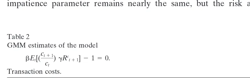
Estimates of the model with transaction costs (aestimated) are displayed in Table 2. As with the estimates of the model with no costs, the estimated parameters are generally significant and have the correct sign. The problem with the impatience parameter remains, however. Thex2statistic for the overidentifying restrictions implies
that the orthogonality conditions are still not rejected by the data.
Table 1
GMM estimates of the model
bEt[(ct11 ct
)gRt11]2150. No transaction costs.
Instrument lags56. Sample: September 1959–June 1989
MA lags b g x2
0 1.0055 24.3299 10.2795
(208.867) (22.5531) 17
2 1.0056 24.2572 11.7402
(201.638) (22.4027) 17
4 1.0047 23.8814 11.9204
(194.434) (22.1805) 17
6 1.0039 23.6380 12.2628
(197.342) (22.1218) 17
GMM estimates of the parameters describing impatience (b) and risk aversion (g) for the Euler Eq (3).t-statistics are in parentheses.x2denotes the value of the statistic for the test of the overidentifying restrictions; degrees of freedom are below.
Instruments: Constant, lagged returns, lagged nondurables consumption growth, and lagged volume detrended by its moving average.
significant role in explaining the relationship between real returns and intertemporal substitution. The way in which volume enters the intertemporal substitution problem strongly suggests that this role relates to transactions costs. The negative estimate also implies that marginal costs decrease in volume, which is sensible given the actual structure of brokerage commission schedules, for example. Also, it implies that funda-mentals (the relationship of consumption growth and returns) will be more in evidence in deeper markets, so that classical asset pricing models should fit better in more active markets, all else equal.
It is also interesting that the estimates of risk aversion (g) are larger for the model with transactions costs. Perhaps this is a reflection of the fact that, as argued above, marginal costs serve as an additional risk factor; this implies a larger market risk premium, which is consistent with greater risk aversion. Alternatively, the adjusted returns, which are more variable than unadjusted returns, require more variable marginal rates of substitution to fit the consumption data.
To investigate the influence of October 1987 on these estimates, the estimation was re-done with data from September 1959 to August 1987 (with six MA lags and six instrument lags). The estimates are different from those estimated through 1989, with estimatedbaround .99, estimatedgabout22.64, and estimatedaabout20.19. All but the estimate ofgare significant at the 1% level. The larger estimate of a in this sample demonstrates that the significance of volume in returns does not stem solely from the October 1987 crash.
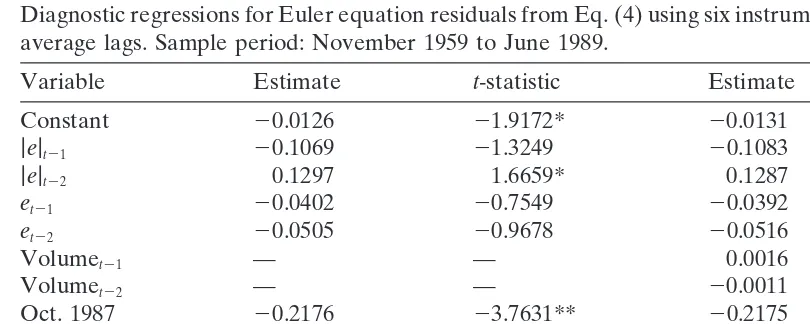
5.2. Specification tests
difference sequence (MDS), as they have a conditional mean of zero. This implies that their level should be unpredictable from lagged variables. Bansal and Viswanathan (1993) exploit this fact to motivate some simple diagnostics for Euler equation residu-als. Following their example, I examine regressions of the Euler equation residuals on lagged residuals, lagged absolute residuals, and lagged volume, none of which should help predict the residual.22 I also include dummy variables for October and
November 1987 (the market crash and its aftermath) and the uniform reduction of brokerage commissions on the New York Stock Exchange as of January 1972, as a specification test on the model.
These tests require picking a particular specification to test. I use the model with six MA lags and six instrument lags. Results for the MDS specification test are in Table 3. Only the dummy variables for the 1987 stock market crash and for the reduction of brokerage fees are significant at usual levels.23This means that the model
cannot account for these structural breaks. October 1987 contains by far the largest negative real return (about221%), so it is not surprising that the model does not fit well to this observation.
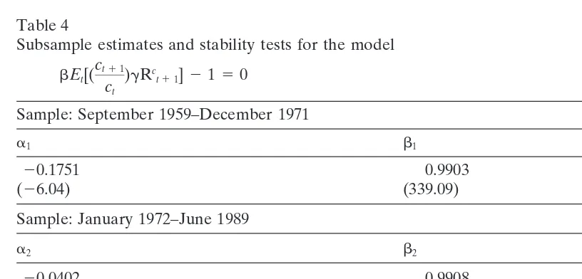
Another specification issue is the constancy of parameters over the sample. The stability of taste parameters in consumption-based asset pricing equations has been the focus of some recent interest.24Likewise, the trading environment implicitly modeled in
f(•) has evolved substantially since the late 1950s. Hence, the stability of these parame-ters ought to be tested. I use the Wald test of Andrews and Fair (1988).25
Table 4 displays the subsample estimates and tests for constant parameters. The impatience parameter remains nearly the same, but the risk aversion parameter
Table 2
GMM estimates of the model
bEt[(ct11 ct
)gRc
t11]2150. Transaction costs.
Instrument lags56. Sample: September 1959–June 1989
MA Lags a b g x2
0 20.1025 1.0071 25.9524 6.8674
(23.8619) (171.32) (22.7592) 16
2 20.0973 1.0079 26.1775 6.7871
(24.3232) (172.15) (22.7966) 16
4 20.0993 1.0074 25.9290 7.3891
(24.6137) (169.30) (22.6977) 16
6 20.1001 1.0070 25.8182 7.5723
(24.9628) (175.81) (22.8076) 16
GMM estimates of the parameters describing impatience (b), risk aversion (g), and marginal transac-tions costs (a) for the Euler Eq. (4).t-statistics are in parentheses.x2denotes the value of the statistic for the test of the overidentifying restrictions; degrees of freedom are below.
Table 3
Diagnostic regressions for Euler equation residuals from Eq. (4) using six instrument lags and six moving-average lags. Sample period: November 1959 to June 1989.
Variable Estimate t-statistic Estimate t-statistic
Constant 20.0126 21.9172* 20.0131 20.7501
|e|t21 20.1069 21.3249 20.1083 21.3290
|e|t22 0.1297 1.6659* 0.1287 1.6188
et21 20.0402 20.7549 20.0392 20.7264
et22 20.0505 20.9678 20.0516 20.9729
Volumet21 — — 0.0016 0.1280
Volumet22 — — 20.0011 20.0892
Oct. 1987 20.2176 23.7631** 20.2175 23.7504**
Nov. 1987 20.1280 22.1010** 20.1275 22.0831**
1972– 0.0226 3.5335** 0.0226 3.5094**
F 5.29** — 4.098** —
(7,348) (9,346)
R2 0.0781 — 0.0728 —
Estimates for a regression of the GMM residuals on lagged residuals (e.), lagged absolute value of residuals (|e.|), lagged trading volume, and dummy variables for October 1987, November 1987, and the reduction of brokerage commissions in 1972.Fdenotes the test statistic for the null hypothesis that the regression coefficients are jointly zero, with degrees of freedom below.
* Significance at the 5% level. ** Significance at the 1% level.
changes sign (and is small and insignificant in both subsamples). Both parameters are smaller than their full-sample values. The marginal cost parameter is significant in both subsamples. It is smaller than the full-sample value (of about 20.1) after the break and larger before. The tests confirm that the joint change in parameters is significant, and the change in the transaction-cost parameter by itself is also significant. It is interesting that the transaction-costs parameter decreases in absolute value after January 1972. This implies a smaller role of volume in returns, since the function f9(•) is closer to zero for any given level of volume. This is consistent with the decrease in transactions costs along with the lowering of NYSE brokerage commissions in January 1972.
Table 4
Subsample estimates and stability tests for the model
bEt[(ct11 ct
)gRc
t11]2150
Sample: September 1959–December 1971
a1 b1 g1
20.1751 0.9903 0.5536
(26.04) (339.09) (1.26)
Sample: January 1972–June 1989
a2 b2 g2
20.0402 0.9908 20.3405
(25.67) (384.41) (20.3406)
Tests for parameter stability
H0:a15 a2,b15 b2,g15 g2 x2(3)53096.3 (p-value,.01) H0:a15 a2 x2(1)53062.3 (p-value,.01)
Subsample estimates and tests for parameter stability for the Eq. (4). Estimates use six MA lags and six instrument lags.
6. Indirect tests
6.1. Volume as a conditioning variable in the risk-return relationship
Estimation of the Euler equation requires strong assumptions about the functional forms for utility and transactions costs. Other questions of specification, such as stability and time-separability, may obscure the results as well. For these reasons, it is useful to compare results from a simpler (and, I hope, more robust) procedure. The next set of tests posit trading volume as a conditioning variable in linear pricing relations. In particular, the relation of risk—here, market risk and consumption risk—to average return across stocks is examined over high-volume and low-volume subsamples. If volume is irrelevant to this relationship, it should look the same in both subsamples.
by sorting returns into high-volume and low-volume months, and fitting separate cross-sectional asset-pricing models to each sample.
The classical tests of the linear asset pricing theory employ a two-stage approach to estimate cross-sectional models of the form
E(rit) 5 l0bi (5)
wherebi is a measure of the riskiness of stockI, l1 is the premium for risk-bearing
over the riskless rate (l0), andritis the return on stockI for periodt.26biand l1may
be scalars or vectors, depending on whether one or many risk factors are priced. For example, in the CAPM,biis the covariance of the return on stockIwith the market
return divided by the variance of the market return, or the slope coefficient in the time-series regression
rit5 ai1 birmt1 eit (6)
wherermtis the return on a stock market index. This suggests the following estimation
strategy: estimate bifor a group of stocks I5 1, . . . ,Nusing time series data as in
Eq. (6), then regress average returns on these estimates to yield estimates ofl1, the
market risk premium. That is, the cross-sectional regression
ri5 l01 l1bˆi1gi (7)
yields estimatesl0and l1. The parameter l1characterizes the tradeoff between risk
and expected return. If increased risk is compensated by increased expected return, then the estimatel1should be positive and significantly different from zero.
Two types of circumstances can give rise to a model such as Eq. (5). Under certain restrictions on preferences or the distribution of returns, for example,biis the slope
coefficient from a regression of stockI’s return on the return on the market portfolio (e.g., the CAPM). Under restrictions on the economy,biis the slope coefficient from
a regression of stock I’s return on real consumption growth (e.g., a variant of the
Consumption CAPM or CCAPM).27
The fundamental question is whether aggregate volume plays any role in the equilib-rium pricing relationship Eq. (5). This question is posed by dividing a sample of stock returns into three parts, corresponding to the months of the 1/3 highest, 1/3 lowest, and 1/3 median aggregate volume on the New York Stock Exchange. The ratio of volume to its 100-day moving average is used to form this ranking, rather than its level. Otherwise, all the high-volume months would come toward the end of the sample, and all the low-volume months toward the beginning; this might confuse shifts due to volume with shifts due to institutional phenomena.28 Relationships as in Eq.
(7) are then examined over the full sample and the high- and low-volume subsamples. If volume is irrelevant to stock returns, the relationship of risk and return, or l1,
should be the same in all three samples.
The estimation procedure is contaminated by errors-in-variables bias, as estimated (rather than population)biare used in the second pass regression. However, because
l1are consistent (as the time-series sample size increases) under moderate restrictions
on the processes governing the time-series behavior of returns.29They are also
asymp-totically normal; the usual ordinary least squares standard errors are inconsistent, though, and here are replaced by standard errors adjusted for estimation error (Shan-ken, 1992).
6.2. Data
Monthly data on individual stock returns for the sample period May 1959 to June 1987 are taken from the CRSP data tape. This sample consists of both NYSE and American Exchange stocks. The period of the market crash of 1987 and months thereafter is excluded from the sample, as the sample is large enough to produce good estimates from this technique without the last few years of data. Individual stock returns are grouped into 50 equally-weighted portfolios on the basis of the previous
month’s size (price times number of shares outstanding).30 Grouping returns into
portfolios reduces the estimation error of the first-pass estimates by decreasing firm-specific variation (which tends to cancel out in portfolios). Grouping by size increases the power of tests based on the cross-sectional regression by assuring that the sample will have a good dispersion of risk and return across portfolios.
Returns on the S&P 500, the equally-weighted CRSP index, and the value-weighted CRSP index are also taken from CRSP. The return on the one-month Treasury bill with maturity closest to one month (Ibbotson & Sinquefeld, 1990) was used as the risk-free rate of return. This was subtracted from all returns series (including the market return rmt) before estimation, as net-risk-free returns are indistinguishable
from real returns at one-month intervals.31This also implies thatl
050. Consumption
of nondurables in 1982 dollars was used for the consumption series.
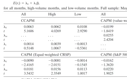
6.3. Results
Table 5 shows the results for the various linear pricing models, with consumption, the S&P 500, the CRSP equally-weighted index, and the CRSP value-weighted index as risk factors (rmt). I find, as do Mankiw and Shapiro (1986) and Chen, Roll, and
Ross (1986), that consumption risk does not explain average return. It is interesting to note that both by itself and combined with the market return, the estimated premium for consumption risk is largest in high-volume months (though still not significant at usual levels).
In contrast, market risk explains average return for high-volume months, with a risk premium significantly different from zero. This is true regardless of how the market portfolio is defined. In low-volume months, however, market risk is no longer significant, and point estimates fall by a factor of 10. The results for all months together are similar to those for high-volume months.
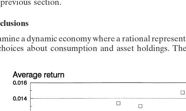
Figs. 1 and 2 Highlight the differences in risk and return in high- and low-volume months. In these figures, the squares show pairs ofbIand r¯Ifor the 50 portfolios and
Table 5
Estimates of linear pricing models
E(ri)5 l01 l1bi
for all months, high-volume months, and low-volume months. Full sample: May 1959–June 1987.
All High Low All High Low
CCAPM CAPM (value-weighted CRSP)
l0 0.0063 0.0062 0.0108 20.0199 20.0196 0.0027
t 5.1606 4.0269 2.9290 21.8419 21.6638 0.1753
lm . . . 0.0255 0.0222 0.0061
t . . . 2.4204 2.0115 0.3774
lc 0.0014 0.0039 20.0013 . . . .
t 0.5148 1.0067 20.5361 . . . .
CAPM (Equal-weighted CRSP) CAPM (S&P 500)
l0 20.0090 20.0081 20.0014 20.0162 20.0207 0.0062
t 22.4165 22.0151 20.1545 21.3620 21.4754 0.4222
lm 0.0181 0.0156 0.0113 0.0220 0.0230 0.0025
t 3.5432 2.3549 1.0017 1.9025 1.7913 0.1670
CAPM (VW)/CCAPM
l0 20.0199 20.0180 20.0014
t 21.8366 21.4284 20.0827
lm 0.0256 0.0209 0.0095
t 2.4177 1.7865 0.5511
lc 0.0010 0.0032 20.0017
t 0.3189 0.7762 20.6668
Estimates of CAPM and Consumption CAPM models over different volume regimes.lmdenotes the estimated market risk premium and lc the estimated consumption risk premium. t denotes the test statistic (asymptotically distributedN(0,1)) for the hypothesis that the corresponding parameter is zero, based on the Shanken (1992) standard error (adjusted for measurement error inbˆ ).
(measured relative to the value-weighted CRSP index) versus average return for high-volume months. Beta varies from about .9 to about 1.4, while average return runs from about 0 to almost 2% per month. Moreover, there is a significant relationship between the two. Fig. 2 shows market beta versus average return in low-volume months. Here, the spread in both risk and return is smaller; beta varies from about .9 to about 1.15, while average return varies from about 0.4% per month to about 1.5% per month. Moreover, the relationship between the two is insignificant (the reader should note that the two plots are not strictly comparable since thex-axes are scaled differently).
Fig. 1. Average return vs. market beta: high-volume months.
are more likely to be obscured by noise trading (through transactions costs). This is consistent with the estimates of declining marginal transaction costs from the model of the previous section.
7. Conclusions
I examine a dynamic economy where a rational representative agent makes intertem-poral choices about consumption and asset holdings. The rational agent operates in
a market with noise traders, whose activities affect the marginal cost of transaction. This implies that trading volume will play a role in determining the real equilibrium prices of assets. The model is amenable to estimation using GMM. Both direct and indirect estimates lend support to a role for volume in equilibrium asset returns. In particular, both imply that variations in volume when average volume is high affect equilibrium returns less than when average volume is low.
In this model, frictions do not eliminate the effects of noise trading on prices; rather, they cause the (marginal-cost) risk associated with noise trading to be priced by rational agents. It is not hard to see why: rational agents, who create the link between fundamentals and asset prices, are subject to transactions costs as well. The resulting equilibrium is not inefficient per se; risk is still correctly priced. However, there is an additional source of risk that will confound analysis that uses traditional tools (such as the CAPM) to assess market equilibrium and the cost of capital. This assertion is consistent with the evidence that the CAPM relationship of return to risk is different in high-volume months than in low-volume months.
Acknowledgments
I am grateful to Erik Benrud, Craig Hiemstra, Jonathan Jones, Robert Flood, Lee Redding, and an anonymous referee for helpful comments.
Notes
1. Karpoff (1987) provides an overview of work on prices and volume through 1987. Redding (1996), LeBaron (1991a and 1991b), Brock (1993), Campbell, Grossman, and Wang (1993), Gallant, Rossi, and Tauchen (1992), Hiemstra and Jones (1994), Lamoreux and Lastrapes (1990), and Antoniewicz (1992) are examples of more recent work.
2. See Niehans (1994), for example.
3. See for example Delong et al. (1990a and 1990b), Campbell, Grossman, and Wang (1993), and Brock (1993).
4. Recent examples are Blume, Easley, and O’Hara (1994) and Easley and O’Hara (1992).
5. See Demsetz (1968) and Epps (1976).
6. These mirror similar considerations of the rate of information transmission as a function of market depth. See Easley and O’Hara (1992).
7. See Black (1986) for a discussion and motivation of the economics of noise trading.
8. See Demsetz (1968) and Cohen et al. (1980).
prices. These are different from the transactions costs implied by the model, which more closely resemble brokerage fees and the bid-asked spread. 10. Similar assumptions are made in the microstructure literature (e.g., Easley &
O’Hara, 1992). Such assumptions mean that the issue of no-trade equilibria can be ignored (Milgrom & Stokey, 1982).
11. One exception might be if agents place market orders that brokers execute with a lag (for example, in a call auction market). The markets examined here (the NYSE and AMEX) are more like continuous auctions than call auctions, though.
12. That is, for a givenv,f(|Dx|v) is the cost of trading|Dx|shares. Quasiconvexity ensures that the budget set is convex.
13. See Sargent (1987, Appendix). 14. For brevity, the algebra is omitted.
15. See Kramer (1994) and Kocherlakota (1996).
16. See Davidson and MacKinnon (1993, pp. 607–614) for details on robust standard errors for GMM models.
17. See Delong et al. (1990a).
18. For a discussion of neural network modeling in econometrics see Granger and Tera¨svirta (1993).
19. While the parameters might be locally identified, Granger and Tera¨svirta (1993, p. 125) point out that neural network functions are not globally identified. 20. Omitting this transformation produced qualitatively similar results (e.g. negative
and significant estimates of a).
21. I am grateful to Craig Hiemstra and Jonathan Jones for providing this data. 22. Bansal and Viswanathan (1993) recommend including lagged absolute values
as a check for neglected nonlinearity. Also, strictly speaking, lagged volume should be orthogonal to the residual because it is used as an instrument. Includ-ing it serves as a second check that the model explains the relationship of volume and returns (e.g., that the failure to reject the overidentifying restrictions is not due to a power problem).
23. A dummy variable for the SEC’s deregulation of minimum brokerage commis-sions on the NYSE (May 1975) was insignificant when added to these regres-sions.
24. See Ghysels and Hall (1990). 25. See Hamilton (1994, pp. 425–427). 26. Shanken (1992) reviews these tests.
27. Mankiw and Shapiro (1986) discuss these two models.
28. The dates associated with high- and low-volume months are scattered through-out the sample. This scheme destroys any serial correlation in the residual, but because such correlation is rarely exploited in this type of test, no real harm is done.
29. See Shanken (1992).
30. The current month’s size was not used as this would induce a spurious correlation between average return and portfolio rank.
References
Andrews, D. W. K., & Fair, R. (1988). Inference in nonlinear econometric models with structural change.
Review of Economic Studies 55, 615–640.
Antoniewicz, R. (1992). A Causal Relationship Between Volume and Return. Mimeo, Federal Reserve Board of Governors.
Bansal, R., & Viswanathan, S. (1993). No arbitrage and arbitrage pricing: a new approach.Journal of Finance 48, 1231–1262.
Black, F. (1986). Noise.Journal of Finance 41, 529–543.
Blume, L., Easley, D., & O’Hara, M. (1994). Market statistics and technical analysis: the role of volume.
Journal of Finance 49, 153–182.
Breeden, D. (1979). An intertemporal asset pricing model with stochastic consumption and investment opportunities.Journal of Financial Economics 71, 265–296.
Brock, W. (1982). Asset prices in a production economy. In J. J. McCall (Ed.),The Economics of Information and Uncertainty(pp. 1–43). Chicago, IL: University of Chicago Press.
Brock, W. (1993). Beyond Randomness: Emergent Noise. Mimeo, Department of Economics, University of Wisconsin.
Campbell, J., Grossman, S., & Wang, J. (1993). Trading volume and serial correlation in stock returns.
Quarterly Journal of Economics 108, 905–939.
Chen, N. F., Roll, R., & Ross, S. (1986). Economic forces and the stock market.Journal of Business 59, 383–403.
Cohen, K. J., Hawawini, G. A., Maier, S. F., Schwartz, R. A., & Whitcomb, D. K. (1980). Implications of microstructure theory for empirical research on stock price behavior.Journal of Finance 35, 249–257. Davidson, R., & MacKinnon, J. G. (1993).Estimation and Inference in Econometrics.New York, NY:
Oxford University Press.
Delong, J., Shleifer, A., Summers, L., & Waldmann, R. (1990a). Noise trader risk in financial markets.
Journal of Political Economy 98, 703–738.
Delong, J., Shleifer, A., Summers, L., & Waldmann, R. (1990b). Positive feedback investment strategies and destabilizing rational speculation.Journal of Finance 45, 379–395.
Demsetz, H. (1968). The cost of transacting.Quarterly Journal of Economics 87, 33–53.
Easley, D., & O’Hara, M. (1992). Adverse selection and large trade volume: the implications for market efficiency.Journal of Financial and Quantitative Analysis 27, 185–208.
Epps, T. W. (1976). The demand for brokers’ services: the relation between security trading volume and transaction cost.Bell Journal of Economics 7, 163–194.
Ferson, W. (1990). Are the latent variables in time-varying expected returns compensation for consump-tion risk?Journal of Finance 45, 397–429.
Gallant, R., Rossi, P., & Tauchen, G. (1992). Stock prices and volume.Review of Financial Studies 5, 199–242.
Ghysels, E., & Hall, A. (1990). Are consumption-based intertemporal capital asset pricing models struc-tural?Journal of Econometrics 45, 121–139.
Granger, C., & Tera¨svirta, T. (1993).Modelling Nonlinear Economic Relationships. Oxford: Oxford University Press.
Hamilton, J. (1994).Time Series Analysis.Princeton NJ: Princeton University Press.
Hansen, L. P. (1982). Large sample properties of generalized method of moments estimators. Economet-rica 50, 1029–1054.
Hansen, L. P., & Singleton, K. (1983). Stochastic consumption, risk aversion, and the temporal behavior of asset returns.Journal of Political Economy 91, 249–268.
Hansen, L. P., & Singleton, K. (1982). Generalized instrumental variables estimation of nonlinear rational expectations models.Econometrica 50, 1269–1286. Erratum (1984) 52, 267–268.
Hiemstra, C., & Jones, J. (1994). Testing for linear and nonlinear granger causality in the stock price-volume relationship.Journal of Finance 49, 1639–1664.
Ibbotson, R., & Sinquefeld R. (1990). Stocks, Bonds, Bills and Inflation: The Past and the Future.
Karpoff, J. (1987). The relation between price changes and trading volume: a survey.Journal of Financial and Quantitative Analysis 22, 109–126.
Kocherlakota, N. R. (1996). The equity premium puzzle: it’s still a puzzle.Journal of Economic Literature 34, 42–71.
Kramer, C. (1994). Macroeconomic seasonality and the january effect.Journal of Finance 49, 1883–1891. Lamoreux, C. & Lastrapes, W. (1990). Heteroskedasticity in stock return data: volume versus GARCH
effects.Journal of Finance 45, 221–229.
LeBaron, B. (1991a). Persistence of the Dow Jones Index on Rising Volume. Mimeo, Social Systems Research Institute, University of Wisconsin.
LeBaron, B. (1991b). Transactions Costs and Correlations in a Large Firm Index. Mimeo, Social Systems Research Institute, University of Wisconsin.
Lucas, R. E. (1978). Asset prices in an exchange economy.Econometrica 46, 1429–1445.
Mankiw, N. G., & Shapiro, M. (1986). Risk and return: consumption beta versus market beta.Review of Economics and Statistics 68, 452–459.
Milgrom, P., & Stokey, N. (1982). Information, trade and common knowledge. Journal of Economic Theory 26, 17–27.
Niehans, J. (1994). Arbitrage equilibrium with transactions costs.Journal of Money, Credit and Banking 24, 249–270.
Ogaki, M. (1993). Generalized Method of Moments: Econometric Applications. In G.S. Maddala, C. R. Rao, and H. D. Vinod (Eds.),Handbook of Statistics (pp. 455–488). Amsterdam: Elsevier Science Publishers.
Redding, L. S. (1996). Noise Traders and Herding Behavior. Mimeo, Department of Economics, Fordham University.
Ross, S. (1976). The arbitrage theory of capital asset pricing.Journal of Economic Theory 13, 341–360. Sargent, T. (1987).Dynamic Macroeconomic Theory.Cambridge: Academic Press.
Shanken, J. (1992). On the estimation of beta-pricing models.Review of Financial Studies 5(1), 1–33. Tsibouris, G. (1993). Emergent Noise in Foreign Exchange Markets. Mimeo, International Monetary