Directory UMM :Data Elmu:jurnal:E:Economics Letters:Vol68.Issue1.Jul2000:

www.elsevier.com / locate / econbase

Generalized bivariate count data regression models

a ,

_*

b

Shiferaw Gurmu

, John Elder

a

Department of Economics, University Plaza, Georgia State University, Atlanta, GA 30303, USA b

Department of Economics, Munroe Hall, Middlebury College, Middlebury, VT 05753, USA Received 16 June 1999; accepted 21 October 1999

Abstract

This paper proposes a flexible bivariate count data regression model that nests the bivariate negative binomial

regression. An application to the demand for health services is given.  2000 Elsevier Science S.A. All rights

reserved.

Keywords: Correlation; Censoring; Unobserved heterogeneity; Bivariate Negbin

JEL classification: C35; I10

1. Introduction

Event counts such as the number of doctor consultations and prescription drug utilization are likely to be jointly dependent. Another example of bivariate counts is the number of voluntary and involuntary job changes. Applications of these models have largely been confined to the bivariate Poisson regression model. This benchmark model imposes the restriction that the conditional mean of each count variable equals the conditional variance. For the common case of overdispersed counts, the bivariate negative binomial model is potentially useful. But this model has mainly been used in the

1

context of panel data .

This paper develops a more general flexible bivariate count regression model based on first-order series expansion of the unknown density of unobserved heterogeneity component. We also extend the approach to estimation of censored bivariate regression models. We apply the method to bivariate models of the demand for health services. The dependent variables are the number of visits to a doctor and the number of visits to non-doctor health professionals. The proposed bivariate model nests the

*Corresponding author. Tel.: 11-404-651-1907; fax:11-404-651-4985.

E-mail address: sgurmu@gsu.edu (S. Gurmu) 1

Gurmu and Trivedi (1994) and Cameron and Trivedi (1998) provide an overview of standard bivariate count models.

bivariate negative binomial model as a special case. In the empirical application, the proposed generalized model dominates existing bivariate models using various criteria for comparing models.

2. The bivariate model

Consider two jointly distributed random variables, Y and Y , each denoting event counts. For1 2 2

observation i (i51,2, . . . ,N ), we observe y , x

h

_{ji ji j}

j

₅₁, where x is a (k_{ji j}31) vector of covariates. The

9

mean parameter associated with yji can be parameterized as uji5exp(xjibj), j51,2, where bj is a (k_j31) vector of unknown parameters. If there is evidence that the dependent count variables y and₁

y are correlated, joint estimation of the underlying equations is desirable. The most widely known2

model is the bivariate Poisson regression model which can be generated by convolutions of Poisson random variables (Kocherlakota and Kocherlakota, 1992). The model restricts the mean to be equal to the variance for each of the respective marginal distributions; E( y_jiux )_ji 5var( y_jiux ) for j_ji 51,2.

As in the univariate case, bivariate count models can be generalized to allow for overdispersion. We consider a bivariate model with unobserved heterogeneity. Let ( yjiux ,jini)|Poisson(u nji i), where ni is the unobserved heterogeneity component with density g(ni). The mixture bivariate density takes the form:

The proposed estimation approach is based on first-degree polynomial expansion of the distribution of unobserved heterogeneity where the leading term in the expansion is the gamma density with parameters a and l. The proposed flexible density is:

a21 a

parameter. The polynomial is squared to ensure non-negativity of the density in (2) . After some algebra, the mixture bivariate density (1) based on specification (2) can be derived as:

y

where:

The log-likelihood can now be constructed readily. As in the univariate mixture Poisson models, we set the mean of the unobserved heterogeneity to unity. This implies the restriction:

1 _Œ] 2

]]

l5 ₂

f

a22r a1r as 12d

g

(5)

11r

The model given in (3) will be referred to as the generalized bivariate negative binomial (GBIVARNB). Thus, the log-likelihood function for the GBIVARNB regression model is +_(w)5

N

oi51 ln f( y , y

s

1i 2iux ) , where f(.) is given in (3) subject to the restriction (5). Herei

d

w consists of the unknown parameters b₁, b₂, a and r.

The model just given can be generalized to truncated and censored jointly dependent count regression models. Censored samples may result when high counts are not observed, or may be imposed by survey design; see, for example, Okoruwa et al. (1988). Thus right censoring is the most common form in the analysis of univariate count models. Suppose that the bivariate counts are right censored at r5(r , r ) so that y1 2 ji51, 2, 3,...r for jj 51,2. Letting f( y , y ;1i 2i w) denote the complete bivariate density (3), the log-likelihood for the right-censored bivariate count model is:

r 21 r 21

N 1 2

+_(w)5

O

_{d ln f( y , y ;}

f

_w)

g

₁f_{12d ln 1}g

F

₂

O O

_{f( y 5l, y 5m;w)}

G

₍₆₎

c i 1i 2i i 1i 2i

i51 l50 m50

where di51 if y falls in the uncensored region, and di50 otherwise.

The proposed approach provides flexible forms for the variances of the y_ji values and the

3

correlation between the dependent variables. The correlation coefficient for model (3) is:

Vu u_{1i 2i}2u u_{1i 2i}

Another advantage of the proposed regression model is that it nests the bivariate negative binomial (BIVARNB) model when r50. Note that, since r50 implies thatCi51, settingCi51 andl5a

in (3) gives the BIVARNB model. The restriction r50 can be used to test for the adequacy of the BIVARNB model using, for example, a score test. As a rough guide, the significance of the t-ratio corresponding to r is indicative of the inadequacy of the BIVARNB regression. In the application section, we also use the Akaike Information Criterion (AIC) to compare the estimated models. A model with a minimum AIC value is to be preferred.

3

3. An application

The data analyzed here were originally employed by Cameron et al. (1988) in their analysis of various measures of health-care utilization using a sample of 5190 single-person households from the 1977–1978 Australian Health Survey. The data are obtained from the Journal of Applied Econo-metrics 1997 Data Archive. Here we model two possibly correlated dependent variables: (1) the number of consultations with a doctor during the 2-week period prior to the survey (Doctorcon); and (2) the number of consultations with non-doctor health professionals (chemist, optician, physiotherap-ist, social worker, district community nurse, chiropodist or chiropractor) during the past 4 weeks (Nondoccon). These utilization measures have two interesting features — overdispersion and a very high proportion of non-users. The mean and the standard deviation of doctor visits are 0.302 and 0.798. The corresponding values for health professionals are 0.215 and 0.965. The frequencies of zero visits in the Doctorcon and Nondoccon samples are 80% and 91%, respectively.

The explanatory variables are as follows: (1) Socio-economic variables — a dummy variable for whether or not the patient is female (Sex), age in years divided by 100 (Age), age-squared (Agesq), and annual income in ten-thousands of dollars (Income); and (2) insurance and health status variables-indicator variable for private insurance coverage (Levyplus), free government insurance cover due to low income (Freepoor), free government coverage due to old age, disability or veteran status (Freerepa), default government Medibank insurance coverage paid for by income levy (Levy), number of illnesses in the past 2 weeks (Illness), number of days of reduced activity in past 2 weeks due to illness or injury (Actdays), general health questionnaire score using Goldberg’s method with high score indicating bad health (Hscore), indicator variable for chronic condition not limiting activity (Chcond1), and indicator variable for chronic condition limiting activity (Chcond2). See Cameron et al. (1988) for summary statistics of the covariates.

An important consideration is whether the two health utilization variables are independent or not. Following a general framework for testing independence in various models summarized in Cameron and Trivedi (1998), p values of tests of independence for Doctorcon and Nondoccon are computed. For example, p values of tests of zero correlation of order one in baseline Poisson and negative binomial models are all less than 2%. There is overwhelming evidence that Doctorcon and Nondoccon are dependent counts, and hence joint estimation is desirable.

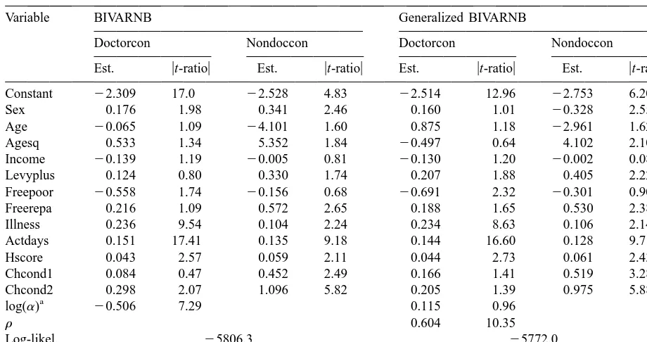
The bivariate Poisson model seems to be inadequate for joint estimation of overdispersed count data. Table 1 presents the maximum likelihood estimates of the BIVARNB and the generalized BIVARNB. The table reveals that the GBIVARNB dominates the BIVARNB model in terms of both the maximized value of the log-likelihood function and the AIC. The GBIVARNB estimates show that recent health status measures (Illness, Actdays) and one of the measures of long-term health status (Hscore) are important determinants of both doctor and non-doctor health professional visits. All of these are significant at 5%. The positive coefficient on the health status insurance variable Levyplus indicates that, relative to the default government Medibank insurance coverage, private insurance is associated with higher use of health services. Further, Non-doctor consultation is responsive to Sex, Age-sq, Chcond1 and Chcond2. The preferred model predicts a convex relationship between Non-doctor health care utilization and age, with a minimum number of visits reached at about age 35. Both health utilization measures are unresponsive to changes in income.

Table 1

Estimates from bivariate models

Variable BIVARNB Generalized BIVARNB

Doctorcon Nondoccon Doctorcon Nondoccon

Est. ut-ratiou Est. ut-ratiou Est. ut-ratiou Est. ut-ratiou

Constant 22.309 17.0 22.528 4.83 22.514 12.96 22.753 6.20

Sex 0.176 1.98 0.341 2.46 0.160 1.01 20.328 2.55

Age 20.065 1.09 24.101 1.60 0.875 1.18 22.961 1.62

Agesq 0.533 1.34 5.352 1.84 20.497 0.64 4.102 2.10

Income 20.139 1.19 20.005 0.81 20.130 1.20 20.002 0.08

Levyplus 0.124 0.80 0.330 1.74 0.207 1.88 0.405 2.22

Freepoor 20.558 1.74 20.156 0.68 20.691 2.32 20.301 0.90

Freerepa 0.216 1.09 0.572 2.65 0.188 1.65 0.530 2.38

Illness 0.236 9.54 0.104 2.24 0.234 8.63 0.106 2.14

Actdays 0.151 17.41 0.135 9.18 0.144 16.60 0.128 9.71

Hscore 0.043 2.57 0.059 2.11 0.044 2.73 0.061 2.43

Chcond1 0.084 0.47 0.452 2.49 0.166 1.41 0.519 3.28

Chcond2 0.298 2.07 1.096 5.82 0.205 1.39 0.975 5.88

a

The coefficients log(a) andr are common to both the Doctorcon and Nondoccon equations.

of some variables such as Sex, Levyplus and Chcond2 in the Doctorcon equation. We also computed the predicted marginal effects of changes in the regressors on the mean number of visits (Footnote 4). Generally the marginal effects are greater in the bivariate models than in the independent Poisson and Negbin models. The difference in the mean effects for various models is likely to be particularly important for significant regressors. The sample average of the correlation between Doctorcon and Nondoccon is 0.019 for bivariate Poisson, and about 0.3 in both the BIVARNB and GBIVARNB models.

4. Conclusion

This paper has developed a generalization of the bivariate negative binomial regression model. In the empirical application, the generalized model dominates existing bivariate models in terms of

4

various statistical criteria . The approach has recently been extended to estimation of multi-factor error multivariate count models.

4

A GAUSS program used in this paper will be made available at the following Web site: http: / / www.gsu.edu /|ecosgg; a

References

Cameron, C., Trivedi, P.K., 1998. Regression Analysis of Count Data, Cambridge University Press.

Cameron, C., Trivedi, P.K., Milne, F., Piggott, J., 1988. A microeconometric model of the demand for health care and health insurance in Australia. Review of Economic Studies LV, 85–106.

Gurmu, S., Rilstone, P., Stern, S., 1999. Semiparametric estimation of count regression models. Journal of Econometrics 88, 123–150.

Gurmu, S., Trivedi, P.K., 1994. Recent developments in event count models: A survey, Discussion Paper No. 261, Thomas Jefferson Center, Department of Economics, University of Virginia.

Kocherlakota, S., Kocherlakota, K., 1992. Bivariate Discrete Distributions, Marcel Dekker, New York.