Journal of Indonesian Economy and Business Volume 24, Number 2, 2009, 145 – 162
THE INDONESIAN INTER-REGIONAL SOCIAL ACCOUNTING
MATRIX FOR FISCAL DECENTRALISATION ANALYSIS
*Budy P. Resosudarmo
Economics College of Asia and the Pacific The Australian National University Canberra, Australia
([email protected]) Ditya A. Nurdianto
Economics College of Asia and the Pacific The Australian National University Canberra, Australia
([email protected]) Djoni Hartono
Faculty of Economics Universitas Indonesia ([email protected])
ABSTRACT
Disparities in development have long been a crucial issue in Indonesia. With regard to the new structure of the Indonesian government, it is of great interest to determine whether Indonesia should further decentralise its budget, and if so, what consequences this would have on the national economy overall. This paper develops a simple economic tool — that is an inter-regional social accounting matrix (IRSAM) multiplier — to analyse the impacts of further decentralising government fiscal policy on regional and national performances.
Our simulations show the following. First, reducing gaps among regional economies and boosting the national economy through a higher fiscal transfer strategy might not achieve the same end; i.e. providing a higher transfer to regions that are lagging behind (Sulawesi and Eastern Indonesia) would most likely reduce gaps among regional economies, but might impact negatively on the national economy overall. Second, in general, a more decentralised fiscal system would benefit households in Sulawesi and Eastern Indonesia, whereas the same cannot be said for Java-Bali, Sumatra, and Kalimantan. Third, impacts of further fiscal transfers on labour income vary considerably depending on the region and type of labour.
Keywords: regional economy, fiscal decentralisation, Social Accounting Matrix
INTRODUCTION
Indonesia is the world’s largest archipe-lagic state and one of the most spatially diverse nations on earth in its resource endowments, population settlements, location of economic activity, ecology, and ethnicity.
Disparity of development status has long been a crucial issue in this country. The regional product of the two richest provinces outside Java, Riau and East Kalimantan, is more than 36 times respectively than that of the poorest province, Maluku. Based on the per capita regional product, East Kalimantan far * The inter-regional social accounting data utilised in this work is built by Budy P. Resosudarmo, Arief A. Yusuf and
Djoni Hartono for the Analysing Pathways to Sustainability in Indonesia project, a collaborative project between
Journal of Indonesian Economy and Business May 146
outstrips the rest of the country, including Java. East Kalimantan is twice as rich as the runner-up province, Riau, and more than 16 times richer than Maluku in terms of per capita regional product. Meanwhile, the range of poverty incidence ranged from 4.61 percent of the population in Jakarta to 40.78 percent in
Papua. Table 1 shows several economic indi-cators across regions in Indonesia.
Due to demands from regions that had fallen behind for larger income transfers and greater authority in constructing their development plans, rapid political change took place a few years after the economic crisis of
Table 1. Indonesia’s Regional Outlook
GDP GDP per Capita
Growth of GDP per Capita
Percentage of Poor People
(2007) (2007) 87-07 (2007)
(current Rp.trillion) (Current Rp.000) (%) (%)
Aceh 73.87 17,489 0.1 26.65
North Sumatra 181.82 14,167 4.7 13.90
West Sumatra 59.80 12,729 4.2 11.90
Riau 210.00 41,412 -0.3 11.20
Jambi 32.08 11,697 3.8 10.27
South Sumatra 109.90 15,655 2.5 19.15
Bengkulu 12.74 7,880 3.2 22.13
Lampung 61.82 8,481 5.3 22.19
Sumatra 742.02 17,979 2.8 18.51
Jakarta 566.45 62,490 5.4 4.61
West Java 528.45 13,103 3.2 13.55
Central Java 310.63 9,593 4.2 20.43
Yogyakarta 32.83 9,560 3.7 18.99
East Java 534.92 14,498 4.1 19.98
Bali 42.34 12,166 4.5 6.63
Java-Bali 2,015.62 16,050 4.1 16.52
West Kalimantan 42.48 10,166 4.5 12.91
Central Kalimantan 27.92 13,765 2.9 9.38
South Kalimantan 39.45 11,613 4.5 7.01
East Kalimantan 212.10 70,119 1.1 11.04
Kalimantan 321.94 25,494 2.8 10.31
North Sulawesi 23.45 10,723 5.7 11.42
Central Sulawesi 21.74 9,074 4.5 22.42
South Sulawesi 69.27 8,996 4.8 14.11
Southeast Sulawesi 17.81 8,768 3.8 21.33
Sulawesi 132.28 9,241 4.7 16.11
West Nusa Tenggara 32.17 7,494 4.9 24.99
East Nusa Tenggara 19.14 4,302 3.7 27.51
Maluku 5.70 4,315 4.2 31.14
Papua 55.37 58,632 13.6 40.78
Eastern Indonesia 112.37 10,210 4.8 28.10
Indonesia (total) 3324.23 16,231 3.8 16.58
2009 Resosudarmo, Nurdianto & Hartono 147 1997: Indonesia drastically shifted from a
highly centralistic government system to a highly decentralised one in 2001. Greater authority is delegated to more than 400 districts and municipalities, in the areas of education, agriculture, industry, trade and investment as well as infrastructure (Alm et al., 2001). Only security, foreign relations, monetary and fiscal policies are still the responsibility of the central government (PP No. 25/2000).
Suddenly leaders of district and city levels of government acquired vast authority and responsibility, including receiving a huge transfer of civil servants from sectoral depart-ments within their jurisdiction. Provincial governments, however, generally remained relatively weak. In the new structure, regional governments received a much larger propor-tion of taxes and revenue sharing from natural extraction activities in their regions. It was common for their budgets to triple after implementation of the decentralisation policy. Yet the issue of regional income per capita disparity has not disappeared. It is of great interest to determine whether Indonesia should decentralise its budget even further and if so, what consequences this would have on the national economy overall. The question is what kind of economic tool is appropriate to analyse the impact of such a decision. It is important that the tool be simple enough for policy-makers to understand the analysis easily but it should also allow for further analysis if required.
An inter-regional computable general equilibrium model might be the best tool to analyse this issue, but it is very complicated and not that easy to implement. This paper argues that an inter-regional social accounting matrix (IRSAM) multiplier technique is simple enough as well as being adequate to analyse the impact of fiscal policy on regional and national performances. Furthermore this paper argues that there is no need to develop a very detailed regional IRSAM, such as a
district or provincial level IRSAM, for this purpose. An IRSAM containing five aggregate regions, namely Sumatra, Java-Bali, Kaliman-tan, Sulawesi and Eastern Indonesia, would be adequate. The benefits of only having five regions, of course, are that it is a relatively simple data system and that the multiplier analysis is simple. This paper will explain what an IRSAM is, how to utilise it, and the light it will shed on the implications of further decentralising government fiscal policy.
The outline of this paper is as follows. The next section, Section 2, describes the funda-mentals of a social accounting matrix and Section 3 those of an IRSAM, as well as deriving the multiple coefficients and explaining their meaning. Section 4 presents the Indonesian five-region IRSAM for 2005. Section 5 provides an analysis of two simple more decentralising fiscal policy scenarios, and finally Section 6 is the conclusion of this paper.
FUNDAMENTALS OF THE SOCIAL ACCOUNTING MATRIX
The social accounting matrix (SAM) is a traditional double accounting economic matrix in the form of a partition matrix that records all economic transactions between agents in the economy, especially between sectors in production blocks, sectors within institutional blocks (including households), and sectors within production factors (Pyatt & Round, 1979; Sadoulet & de Janvry, 1995; Hartono & Resosudarmo, 1998). It is a solid database system, since it summarises all transaction activities in an economy within a given time period, thus giving a general picture of the socio-economic structure in an economy and illustrating the income distribution situation.
SAM is also an important analysing tool because: (1) its multiplier coefficients can properly describe economic policy impacts on
a household’s income, hence illustrating the
Journal of Indonesian Economy and Business May 148
simple, thus it can be easily applied to various countries.
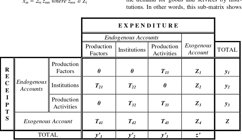
The basic framework of SAM is a 4x4 partition matrix as shown in Figure 1. The accounts in SAM are grouped into endogenous and exogenous accounts. The main endo-genous accounts are divided into three blocks: production factor, institutional, and production activity blocks. The row shows income, while the column shows expenditure. Sub-matrix Tij (or Zi) shows the income of the account in row i from the account of column j. Vector yi (or z) shows the total incomes of all accounts, and vector yj (or z) shows the total expenditure account of all accounts. In addition, SAM requires that vector yiis the same as vector yj, or in other words yj is a transpose of yi, for every i = j. The relations in Figure 1 can be written as (Defourny and Thorbecke, 1984):
y = A y + x [1]
where:
y = vector of total income
x = vector whose members are
xm = n zmn where zmn Zi
A = matrix whose members are
amn = tmn/yn where tmn Tij and yn yj
As an illustration, sub-matrix T13 in Figure 1 shows the amount of production factors used in production activities, which equates to the value added in the production sector, e.g. wages and salaries paid for the use of labour in production activities. Meanwhile, sub-matrix
T21 shows the transfer payment from pro-duction factors to various institutions, namely households, the government, and firms. For example, some farmers in the agricultural sector belong to the small-farmer association; as such, a certain amount of funds will flow from farmers as a production factor to the association as an institution. Sub-matrix T22 shows transfer payments between institutions, such as subsidy payments from the govern-ment or from firms to households as well as transfer payments from one household to another.
On the other hand, sub-matrix T32 shows the demand for goods and services by insti-tutions. In other words, this sub-matrix shows
E X P E N D I T U R E
Endogenous Accounts
Exogenous Account
Production
Factors Institutions
Production
Activities TOTAL
R E C E I P T S
Production
Factors 0 0 T13 Z1 y1
Endogenous
Accounts Institutions T21 T22 0 Z2 y2
Production
Activities 0 T32 T33 Z3 y3
Exogenous Account T41 T42 T43 Z4 Z
TOTAL y’1 y’2 y’3 z’
Source: Thorbecke (1985)
2009 Resosudarmo, Nurdianto & Hartono 149 the amount of money paid by institutions to
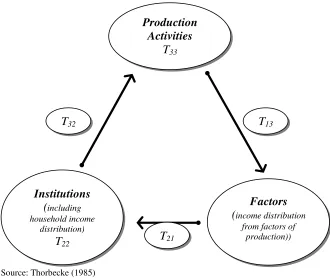
the production sector to buy the goods and services consumed. As for sub-matrix T33, it shows the intra- and inter-industry demand for goods and services, specifically in the production sector. Lastly, aside from the sub-matrices aforementioned, SAM also records economic activities in the financial sector as well as economic transactions with foreign countries. Figure 2 illustrates how an econo-mic activity occurs within an economy.
In general, SAM also provides infor-mation on the social structure within an economy, particularly information related to production structure, production factor condi-tions, household income distribution, and expenditure patterns of institutions. Accor-dingly, SAM is the best approach to generate a general equilibrium analysis (Thorbecke, 1985).
INTER-REGIONAL SAM (IRSAM)
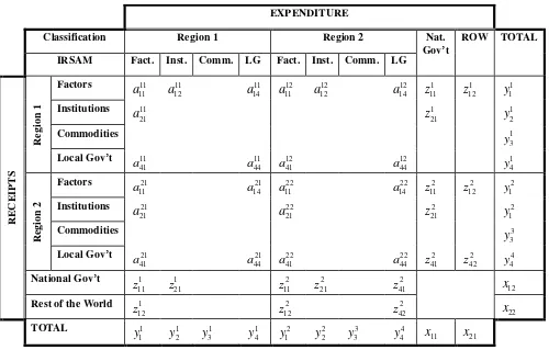
A similar social accounting matrix can also be constructed on a regional level, or in other words, the economy can be divided into separate sub-national economies or regions. In this model, blocks within a region in the economy may receive transfers from various blocks in other regions, albeit still in the same country. Likewise, blocks within a region may also send payments to other blocks outside the region. In order to know how these regions are inter-connected, it is necessary to develop a table such as the one shown in Figure 3. For the time being, transactions are limited to those conducted between two regions of the same country, in other words, the country is divided into two separate regions.
Production
Activities
T
33Institutions
(including
household incomedistribution)
T
22Factors
(income distribution
from factors of production))
T
13T
21T
32Source: Thorbecke (1985)
J
Classification Region 1 Region 2
IRSAM Fact. Inst. Comm. LG Fact. Inst. Comm. LG
2009 Resosudarmo, Nurdianto & Hartono 151 and services that are bought from all blocks in both regions. Variables within the endogenous accounts matrix are written as follows:
rs ij
a where i,j = 1,…,n; r,s = 1,2 [2]
If aij11A11;aij22A22;a12ij A12and aij21A21
then the endogenous accounts matrix can be illustrated in a block matrix form as follows:
block flows between region 1 and region 2.
If national government and the rest of the world (exogenous) accounts are also aggregated and regionally separated as the inter-block flows then equation [1] can be re-written in the following form:
can be written as follows:
in region 1 grows as a result of an increase in
the exogenous accounts, the growth will cause an increase in available resources for use in
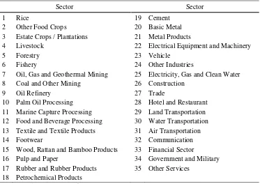
The Indonesian Inter-Regional Social Accounting Matrix constructed for this work consists of five regions: Sumatra, Java-Bali, Kalimantan, Sulawesi and Eastern Indonesia. Within each region, there are 35 production sectors (See Table 2), 16 labour classifications (8 formal and 8 informal) (See Table 3), 2 types of capital (land and capital), 2 types of household (rural and urban), 2 types of other institutions (local government and corporate) and other accounts such as local tax and subsidy and inventory. At the national level there are 3 types of capital accounts (central, local and private capital accounts), central government accounts and other accounts such as tax and subsidy.1
The 2005 IRSAM table for Indonesia is mainly based on the data provided by the 2005 IRIO table. Additional data are used to complete the IRSAM table, including: (i)
National Socio-Economic Survey
(SUSENAS); (ii) National and Regional Balance of Payments; (iii) Current Account; (iv) Population Census; (v) National Labor Force Survey (SAKERNAS); (vi) Special Survey on Household Investment and Savings (SKTIR); (vii) Propinsi dalam Angka; (viii) Indonesian Statistics; and (ix) Statistik Kesejahteraan Rakyat. These sources provide
1 Please contact Budy P. Resosudarmo at
Journal of Indonesian Economy and Business May 152
the data needed for the 2005 Indonesian IRSAM table, which in its summary version can be seen as Figure 4.
Based on the above table, sub-matrix Tij shows the payment flow from account j to account i. As an example, sub-matrix T1,4 shows the added value generated by the
production sector as compensation for producing commodities in Sumatra, such as wage and salary paid out for labour usage. Sub-matrices T2,1 and T3,1 show the institu-tional factor income in Sumatra, namely households, firms, and the regional govern-ment.
Table 2. Sectors in the Indonesian Inter-Regional SAM Table
Sector Sector
1 Rice 19 Cement
2 Other Food Crops 20 Basic Metal
3 Estate Crops / Plantations 21 Metal Products
4 Livestock 22 Electrical Equipment and Machinery
5 Forestry 23 Vehicle
6 Fishery 24 Other Industries
7 Oil, Gas and Geothermal Mining 25 Electricity, Gas and Clean Water 8 Coal and Other Mining 26 Construction
9 Oil Refinery 27 Trade
10 Palm Oil Processing 28 Hotel and Restaurant 11 Marine Capture Processing 29 Land Transportation 12 Food and Beverage Processing 30 Water Transportation 13 Textile and Textile Products 31 Air Transportation
14 Footwear 32 Communication
15 Wood, Rattan and Bamboo Products 33 Financial Sector
16 Pulp and Paper 34 Government and Military
17 Rubber and Rubber Products 35 Other Services
18 Petrochemical Products
Source: Authors' own classification.
Table 3. Labour Classifications in the Indonesian Inter-Regional SAM Table
Labour Classification Labour Classification
1 Formal Rural Agricultural Labour 9 Informal Rural Agricultural Labour 2 Formal Urban Agricultural Labour 10 Informal Urban Agricultural Labour 3 Formal Rural Manual Labour 11 Informal Rural Manual Labour 4 Formal Urban Manual Labour 12 Informal Urban Manual Labour 5 Formal Rural Clerical Labour 13 Informal Rural Clerical Labour 6 Formal Urban Clerical Labour 14 Informal Urban Clerical Labour 7 Formal Rural Professional Labour 15 Informal Rural Professional Labour 8 Formal Urban Professional Labour 16 Informal Urban Professional Labour
2009
R
eso
su
d
a
rm
o
, Nur
d
ia
nto
&
H
a
rto
no
153
Classification Sumatra . . . Eastern Indonesia
IRSAM 2005 1 2 3 4 5 6 7 8 9 10 11 12 13 14 15 16 17 18 19
Factors 1 T1,4 T1,19
Households 2 T2,1 T2,2 T2,3 T2,6 T2,7 T2,8 T2,11 T2,12 T2,13 T2,17 T2,19
Other Institutions 3 T3,1 T3,2 T3,3 T3,5 T3,6 T3,7 T3,8 T3,11 T3,12 T3,13 T3,17 T3,19
Commodity 4 T4,2 T4,3 T4,4 T4,5 T4,7 T4,8 T4,9 T4,10 T4,12 T4,13 T4,14 T4,15 T4,16 T4,17 T4,19
S
u
m
a
tr
a
Other Accounts 5 T5,4 T5,16
Factors 6 T6,9 T6,19
Households 7 T7,1 T7,2 T7,3 T7,6 T7,7 T7,8 T7,11 T7,12 T7,13 T7,17 T7,19
Other Institutions 8 T8,1 T8,2 T8,3 T8,6 T8,7 T8,8 T8,10 T8,11 T8,12 T8,13 T8,17 T8,19
Commodity 9 T9,2 T9,3 T9,4 T9,5 T9,7 T9,8 T9,9 T9,10 T9,12 T9,13 T9,14 T9,15 T9,16 T9,17 T9,19
.
.
.
Other Accounts 10 T10,9 T10,16
Factors 11 T11,14 T11,19
Households 12 T12,1 T12,2 T12,3 T12,6 T12,7 T12,8 T12,11 T12,12 T12,13 T12,17 T12,19
Other Institutions 13 T13,1 T13,2 T13,3 T13,6 T13,7 T13,8 T13,11 T13,12 T13,13 T13,15 T13,17 T13,19
Commodity 14 T14,2 T14,3 T14,4 T14,5 T14,7 T14,8 T14,9 T14,10 T14,12 T14,13 T14,14 T14,15 T14,16 T14,17 T14,19
E
a
s
te
rn
In
d
o
n
e
s
ia
Other Accounts 15 T15,14 T15,16
Capital Accounts 16 T16,2 T16,3 T16,7 T16,8 T16,12 T16,13 T16,17 T16,19
National Government 17 T17,1 T17,2 T17,3 T17,4 T17,6 T17,7 T17,8 T17,9 T17,11 T17,12 T17,13 T17,14 T17,17 T17,18 T17,19
Commodity Import 18 T18,2 T18,3 T18,4 T18,7 T18,8 T18,9 T18,12 T18,13 T18,14 T18,16 T18,17
Rest of the World 19 T19,1 T19,2 T19,3 T19,6 T19,7 T19,8 T19,11 T19,12 T19,13 T19,18
Journal of Indonesian Economy and Business May 154
In other words, these matrices record income transfers from factors of production to institutions. Sub-matrices T2,2, T2,3, T3,2, and T3,3 show inter-institutional transfers, such as household subsidies from the government or firms and financial transfers from one house-hold to another. Sub-matrices T4,2 and T4,3 show institutional demands for goods and services, in other words, these sub-matrices represent payments made by institutions to the production sector for goods and services that they consume. Sub-matrix T4,4 shows the demand for goods and services within the production sector, also known as local intermediate input.
In the 2005 Indonesian IRSAM table above, only commodity accounts (rows/ columns 4, 9, and 14 in Figure 4) are taken from the 2005 Indonesian IRIO table, namely sub-matrices T4,j, T9,j, T14,j, Ti,4, Ti,9, and Ti,14, whereas other sub-matrices are derived from other sources. Basically, the construction of an
IRSAM table begins by using a region’s, in this case Sumatra’s, income and expenditure
accounts to present both domestic and foreign transactions. The same method is used for other regions, such that intra- and inter-regional transactions are recorded as well as other domestic transactions, e.g. capital and national government accounts, and foreign transactions. The following section fully describes the construction of the IRSAM table starting with the income and expenditure accounts in Sumatra and closing with foreign transactions.
Note for the case of Sumatra, sub-matrix
T4,2 represents the income account of the production sector. Thus, this sub-matrix shows the payment for all goods and services produced in Sumatra bought by households in Sumatra, whereas sub-matrices T4,7 and T4,12 show the payments for all goods and services produced in Sumatra bought by households in other regions. Meanwhile, sub-matrix T4,3
shows Sumatra’s regional government
procurement for Sumatran goods and services,
while sub-matrices T4,8 and T4,13 show Sumatran goods and services procured by other regional governments. Sub-matrix T4,4 shows industrial, or the production sector’s, purchase of goods and services within Sumatra, whereas sub-matrices T4,9 and T4,14 show the purchase of Sumatran goods and services by industries in other regions. Sub-matrix T4,5shows the purchase of goods and services produced in Sumatra by industries within Sumatra for inventory purposes, unlike sub-matrices T4,10 and T4,15, which show the purchase of goods and services produced in Sumatra by industries outside Sumatra. Sub-matrix T4,16 represents the purchase of goods and services produced in Sumatra by various institutions, specifically investment purchases by the national and regional governments as well as the public. Sub-matrix T4,17shows the national government procurement of goods and services produced in Sumatra, while sub-matrix T4,19presents foreign purchase of goods and services produced in Sumatra, or exports. Note that the 2005 Indonesian IRIO table is used to obtain the value for the above-mentioned sub-matrices.
2009 Resosudarmo, Nurdianto & Hartono 155 Again, all of the above values can be obtained
from the 2005 Indonesian IRIO table.
The following explains income and expenditure accounts for factors of production, households, other institutions, other accounts, and exogenous accounts. The discussion focuses only on the sub-matrices that have not been mentioned previously as the data do not come from the 2005 Indonesian IRIO table, but are obtained from the National Socio-Economic Survey (SUSENAS), National and Regional Balance of Payments, National Current Accounts, Population Census, National Labor Force Survey (SAKERNAS), Special Survey on Household Investment and Savings (SKTIR), Propinsi dalam Angka, Indonesian Statistics, and Statistik Kesejah-teraan Rakyat.
In the case of Sumatra, the income account for factors of production, sub-matrix
T1,19, presents the income received by the region from the use of its factors of production abroad as recorded in the National Current Accounts. As for the household income account, sub-matrix T2,1 shows the income earned by households; i.e. rural and urban households in Sumatra, from factors of production within the region, whereas sub-matrices T2,6 and T2,11show the income earned from factors of production located outside Sumatra. Sub-matrices T2,2, T2,7, and T2,12 show the inter-household transfers from both within and outside Sumatra. Meanwhile, sub-matrix
T2,3 presents the household income in Sumatra from the regional government and firms in Sumatra, while sub-matrices T2,8 and T2,13 present the household income in Sumatra from firms in other regions. Sub-matrix T2,17 shows the household income transfer in Sumatra from the national government, and lastly, sub-matrix T2,19shows the household income from foreign transfers.
Furthermore, the income account for other institutions, represented by sub-matrix T3,1, shows the transfer of payments from capital and land factors of production in Sumatra to
the regional government and firms in the region. Meanwhile, sub-matrices T3,6 and T3,11 show the transfer of payments from capital and land factors of production located outside Sumatra to firms in Sumatra. Sub-matrix T3,2
presents Sumatra’s regional government
income received for households in Sumatra, while sub-matrices T3,7 and T3,12 show
Sumatra’s regional government income from
households in other regions. Sub-matrix T3,3
shows the regional government and firms’
income from firms within Sumatra (intra-regional transfers between institutions), whereas sub-matrices T3,8 and T3,13show the
regional government and firms’ income in
Sumatra from firms in other regions. Sub-matrix T3,5 presents Sumatra’s regional government income from regional taxes, while sub-matrices T3,17 and T3,19 present income transfers to Sumatra’s regional government from the national government and abroad, respectively.
As for the income account of other accounts, sub-matrix T5,4 displays income earned from indirect taxes of various production activities in Sumatra, whose value makes up a part of the income received by the national government from indirect taxes of production activities in Sumatra. Meanwhile, sub-matrix T5,16 displays the regional inventory in Sumatra from the national government and public sector.
Journal of Indonesian Economy and Business May 156
Sumatra to firms outside the region. Finally, sub-matrix T17,1 and T19,1 present payment transfers from the use of factors of production in Sumatra to the national government and abroad, respectively.
For the expenditure account of house-holds, sub-matrix T2,2 shows the payment transfers between households within the same region, in this case Sumatra. Sub-matrices T7,2 and T12,2 show payment transfers between households in different regions, specifically from households in Sumatra to households in other regions. Sub-matrix T3,2 presents the payment transfers between institutions within Sumatra, such as a transfer from a household to the regional government. Similarly, sub-matrices T8,2 and T13,2 show the payment transfers between institutions in different regions, specifically from Sumatra to other regions. Sub-matrix T4,2 displays the demand for goods and services by households within Sumatra, in other words, purchases made by households from the production sector for goods and services that they consume. Sub-matrices T9,2and T14,2 shows the same thing as sub-matrix T4,2 albeit for goods and services derived from the production sector in other regions. Sub-matrices T16,2, T17,2, T18,2, and T19,2, respectively, show household savings in Sumatra, household income tax paid to the national government, payment for imported goods and services, and foreign transfers.
With regard to the expenditure account of other institutions, sub-matrix T2,3 shows the payment transfers between institutions within Sumatra, in this case, payments from the regional government and firms to households. Meanwhile, sub-matrices T7,3 and T12,3 show the transfers from firms in Sumatra to households in other regions. As for sub-matrix
T3,3, it shows transfers between institutions in Sumatra, such as transfers from firms to the regional government as well as transfers within the regional government. Sub-matrices
T8,3 and T13,3 illustrate the payment transfers between different regions, for example, from
firms in Sumatra to other regional govern-ments and firms outside Sumatra. Sub-matrix
T4,3 represents the demand for goods and services produced in Sumatra by institutions in Sumatra, in other words, this sub-matrix shows the purchasing value to the production sector of goods and services bought by firms in Sumatra. Sub-matrices T9,3and T14,3, on the other hand, shows the same thing as sub-matrix T4,3 except that the goods and services are produced in other regions. Sub-matrices
T16,3, T17,3, T18,3, and T19,3, respectively, show firms and regional government savings in Sumatra, tax payments from firms in Sumatra to the national government, payments from the regional government to the national govern-ment, purchase of imported goods and services by the regional government, and foreign transfers from the regional government and firms in Sumatra. As for the other accounts, sub-matrix T3,5 represents payments received by the regional government of Sumatra from taxes. Sub-matrices T4,5, T9,5,and T14,5 repre-sent payment transfers on commodities used for inventory purposes both within and between regions.
Last to be discussed are the accounts related to exogenous variables, namely capital accounts, national government accounts, imports, and the rest of the world accounts. Sub-matrix T18,16 represents investments made by the regional government, national govern-ment, and private sector for imported goods and services from abroad. Sub-matrix T16,17
shows the national government’s savings,
2009 Resosudarmo, Nurdianto & Hartono 157 government, and firms, while sub-matrix T17,19
shows transfers abroad by the national government.
FISCAL DECENTRALISATION
In this section, two simple scenario simulations will be conducted related to fiscal decentralisation policies in which each local government will receive a greater fiscal allocation. In these scenarios, the central government will increase its transfers to local governments through a balanced fund or a general allocation fund. The central govern-ment has at least two options in order to allocate the budget for each region. First,
increase each regional government’s budget
proportionally to its current budget; or second, increase transfers to each regional government by giving additional lump-sum funds. This section then provides typical analysis per-formed using an IRSAM multiplier calcu-lation, particularly observing the impacts of these two options on both national and regional economic performances; i.e. national, regional and sectoral outputs as well as labour household incomes for various classifications.
Accordingly, equation (5) is applied to the 2005 IRSAM for Indonesia to effect the two simulations mentioned above. The exogenous accounts are capital accounts of local govern-ment, central government and the private sector, central government accounts which are indirect tax, subsidy and government expen-diture, export and import, and rest of the world accounts. The rest become endogenous accounts.
In the first simulation (SIM1), each
regional government’s budget is increased by
10 percent proportional to its current budget; and in the second simulation (SIM2), each
regional government’s budget is increased by
giving an additional equal lump sum transfer.
It is important to note that under both scenarios, the additional transfers to regional governments equate to the same amount of funding. The implication is that the central government expenditure will be reduced by an equal amount in both simulations.
The typical ultimate goal of an analysis using a SAM or IRSAM is to understand what impacts a policy creates on household incomes. This section using the two scenario simulations will provide an example of how to observe the impact of a policy on household incomes. Nevertheless, to understand why the impact of a policy on household incomes is as such, one should observe the impact of that policy mostly on labour incomes (though capital incomes are also important) and before that on sectoral performances or outputs. This section hence will observe the impacts of the two decentralisation policy scenarios on labour incomes and sectoral outputs. The sequence presented will be as follows. First, this section presents the changes in sectoral outputs due to those policies. Second, based on what has happened to sectoral output, this section observes the changes in labour incomes and finally to household incomes.
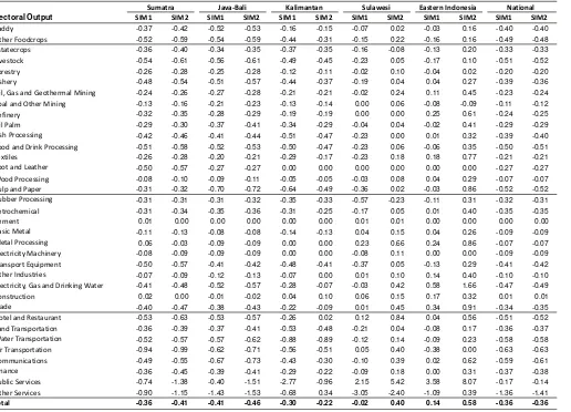
1. Sectoral Performance
J
o
ur
na
l o
f I
nd
o
nes
ia
n E
co
no
m
y
a
nd
B
us
ines
s
Ma
y
158
Sectoral Output SIM1 SIM2 SIM1 SIM2 SIM1 SIM2 SIM1 SIM2 SIM1 SIM2 SIM1 SIM2
Paddy -0.37 -0.42 -0.52 -0.53 -0.16 -0.15 -0.07 0.02 -0.03 0.16 -0.40 -0.40
Other Foodcrops -0.52 -0.59 -0.54 -0.59 -0.44 -0.31 -0.15 0.22 -0.16 0.16 -0.49 -0.48
Estatecrops -0.36 -0.40 -0.34 -0.35 -0.37 -0.35 -0.16 -0.08 -0.13 0.20 -0.33 -0.33
Livestock -0.54 -0.61 -0.56 -0.61 -0.49 -0.45 -0.23 0.05 -0.17 0.10 -0.51 -0.52
Forestry -0.26 -0.28 -0.25 -0.28 -0.12 -0.11 -0.02 0.10 -0.04 0.02 -0.20 -0.20
Fishery -0.48 -0.54 -0.51 -0.57 -0.44 -0.37 -0.19 0.04 0.04 0.27 -0.39 -0.36
Oil, Gas and Geothermal Mining -0.24 -0.26 -0.27 -0.28 -0.21 -0.21 -0.02 0.24 0.11 0.45 -0.23 -0.24
Coal and Other Mining -0.13 -0.16 -0.21 -0.23 -0.13 -0.14 0.00 0.06 -0.08 -0.09 -0.11 -0.12
Refinery -0.32 -0.35 -0.28 -0.29 -0.19 -0.19 0.00 0.00 0.25 0.61 -0.24 -0.25
Oil Palm -0.29 -0.30 -0.37 -0.41 -0.34 -0.29 -0.04 0.04 -0.02 0.41 -0.29 -0.29
Fish Processing -0.42 -0.46 -0.41 -0.44 -0.51 -0.47 -0.23 0.00 0.01 0.32 -0.39 -0.40
Food and Drink Processing -0.51 -0.58 -0.52 -0.53 -0.50 -0.47 -0.23 0.06 -0.06 0.35 -0.50 -0.51
Textiles -0.26 -0.28 -0.20 -0.21 -0.29 -0.17 -0.23 0.18 0.18 0.77 -0.21 -0.21
Foot and Leather -0.50 -0.57 -0.27 -0.27 0.00 0.00 0.00 0.00 0.00 0.00 -0.27 -0.27
Wood Processing -0.08 -0.10 -0.09 -0.11 -0.05 -0.05 -0.03 0.08 0.04 0.29 -0.07 -0.07
Pulp and Paper -0.31 -0.32 -0.70 -0.72 -0.64 -0.49 -0.36 0.02 -0.03 0.86 -0.52 -0.52
Rubber Processing -0.31 -0.31 -0.31 -0.32 -0.35 -0.33 -0.57 -0.23 -0.11 0.31 -0.32 -0.31
Petrochemical -0.31 -0.34 -0.35 -0.36 -0.31 -0.25 -0.17 0.05 0.01 0.40 -0.35 -0.35
Cement 0.01 0.00 0.00 0.00 0.00 0.00 0.01 0.01 0.00 0.00 0.00 0.00
Basic Metal -0.11 -0.13 -0.08 -0.08 -0.14 -0.13 0.04 0.15 0.04 0.26 -0.09 -0.09
Metal Processing 0.06 -0.03 -0.09 -0.09 0.00 0.00 0.23 0.66 0.24 0.86 -0.07 -0.07
Electricity Machinery -0.08 -0.09 -0.09 -0.09 0.00 0.00 -0.08 0.11 0.00 0.00 -0.09 -0.09
Transport Equipment -0.50 -0.57 -0.41 -0.42 -0.48 -0.41 -0.37 0.05 -0.13 0.29 -0.41 -0.42
Other Industries -0.07 -0.09 -0.12 -0.13 -0.07 0.00 0.01 0.10 0.14 0.40 -0.10 -0.10
Electricity, Gas and Drinking Water -0.41 -0.48 -0.52 -0.57 -0.28 -0.07 -0.03 0.42 0.58 1.66 -0.47 -0.49
Construction 0.02 0.00 -0.01 -0.02 0.04 0.10 0.06 0.15 0.17 0.32 0.01 0.01
Trade -0.40 -0.47 -0.38 -0.43 -0.22 -0.09 0.01 0.45 0.34 0.91 -0.34 -0.35
Hotel and Restaurant -0.53 -0.63 -0.53 -0.57 -0.26 0.02 0.12 0.84 0.04 0.56 -0.51 -0.52
Land Transportation -0.36 -0.39 -0.37 -0.41 -0.53 -0.48 -0.21 0.04 -0.08 0.17 -0.36 -0.37
Water Transportation -0.52 -0.57 -0.57 -0.62 -0.88 -0.89 -0.12 0.14 -0.09 0.23 -0.58 -0.58
Air Transportation -0.94 -0.99 -0.62 -0.71 -0.56 -0.51 0.05 0.40 -0.38 0.00 -0.63 -0.63
Communications -0.49 -0.55 -0.67 -0.73 -0.43 -0.30 -0.10 0.39 0.02 0.62 -0.59 -0.61
Finance -0.36 -0.45 -0.39 -0.41 -0.29 -0.22 -0.09 0.18 0.00 0.31 -0.37 -0.38
Public Services -0.74 -1.38 -0.40 -1.51 -2.77 -0.96 2.15 5.42 3.58 8.07 -0.17 -0.14
Other Services -0.90 -1.15 -1.43 -1.53 -0.68 0.34 -3.05 -2.40 -1.09 0.39 -1.36 -1.41
Total -0.36 -0.41 -0.41 -0.46 -0.30 -0.22 -0.02 0.40 0.14 0.58 -0.36 -0.36
Sulawesi Eastern Indonesia National
Sumatra Java-Bali Kalimantan
Table 4. Changes in Sectoral Output (in %)
2009 Resosudarmo, Nurdianto & Hartono 159 Regionally, the impacts of these two
decentralisation scenarios are quite different. In SIM 1, the respective economies of Sumatra, Java-Bali, Kalimantan, and Sulawesi decreases in their aggregated sectoral output by 0.36%, 0.41%, 0.30%, and 0.02%; whereas the aggregated sectoral output of Eastern
Indonesia’s economy actually increases by
0.14%. The sectoral output declines in Sumatra, Java-Bali, Kalimantan and Sulawesi are mainly caused by the relatively large reduction of output in the following sectors: air transportation, public services, and other services for the case of Sumatra; other services as well as pulp and paper for Java-Bali; water transportation and public services for Kalimantan; and other services and rubber processing for Sulawesi.
Meanwhile, in SIM 2, the respective eco-nomies of Sumatra, Java-Bali, and Kalimantan decrease in their aggregated sectoral output by 0.41%, 0.46%, and 0.22%; whereas the aggre-gated sectoral outputs of Sulawesi and Eastern Indonesia increase by 0.40% and 0.58% respectively. Please note that the result for Sulawesi in SIM 2 is different from that in SIM1.
The sectoral output declines in these three regions are mostly due to reductions in the following sectors: air transportation, public services, and other services for the case of Sumatra; air transportation, public services, other services, as well as pulp and paper for Java-Bali; and water transportation and public services for Kalimantan.
The varying effects on the sectoral output of each regional economy can be explained through the following argument; when the central government increases its transfers to regional governments, the central government has to reduce its own expenditure. In this case, consumption expenditure or expenditure on goods and services is expected to decrease. This tends to have a contractionary effect on the economy through the decline in demand for commodities. On the other hand, each
regional government after receiving an addi-tional transfer from the central government increases its demand for consumption expen-diture. This tends to have an expansionary effect on the economy. Whether total demand declines or not depends on which force is stronger. It is important to note at this point that the impact on each region also depends on the nature of inter-regional trade. Regions that supply many goods and services to the central government are expected to be more heavily affected, whereas others are not. As such, in the cases of Sumatra, Java-Bali, and Kaliman-tan, the contractionary effect is greater than the expansionary effect such that the net effect is a reduction in the sectoral outputs of these regions. As can be expected, these three regions supply relatively larger amounts of goods and services to the central government than do Sulawesi and Eastern Indonesia.
Comparing the above two simulations, additional transfer funds in the second simulation mean much higher incomes for the regional governments of Sulawesi and Eastern Indonesia. Accordingly, expenditure consump-tions in these two regions are higher in the second simulation than in the first. As such, sectoral outputs in these two regions increase because the expansionary effect of these regions is greater than the contractionary effect of the central government.
2. Impacts on Labour Income
Journal of Indonesian Economy and Business May 160
sector as well as other services in Kalimantan in the second simulation. Meanwhile, the aggregated sectoral output in each of these three regions also contracts, such that the net effect on workers is negative. Note that the largest negative impact is felt by the formal professional worker in both rural and urban areas in Kalimantan in the first simulation as sectoral output of public services suffers the largest contraction. The largest negative impact is also felt by the formal professional worker in Sumatra and Java-Bali due to a relatively large contraction in the public sector and other services.
Unlike the previous three regions, not every worker in Sulawesi and Eastern Indonesia is adversely affected; in fact, all workers enjoy a positive income effect in the second simulation, except for informal manual workers in both rural and urban areas in Sulawesi. Based on the first simulation, with the exception of the formal clerical and formal professional workers, all other labour types are also adversely affected as almost all sectors undergo a contraction in Sulawesi. Never-theless, a few sectors expand through an increase in output, namely the metal pro-cessing sector, hotel and restaurant sector as well as public services.
Based on the second simulation, the negative impact felt by the informal manual
worker in both rural and urban areas in Sulawesi is mainly caused by a contraction in the rubber processing sector. Whereas based on the first simulation, the negative impact felt by the formal and informal agricultural workers as well as the informal manual worker in both rural and urban areas in Eastern Indonesia is mainly due to contractions in the following sectors: other foodcrops, estate crops, livestock, rubber processing, transport equipment, and air transportation.
As for the positive impact, the formal clerical worker in both rural and urban areas in Sulawesi and Eastern Indonesia is the most positively affected labour type. This positive impact, particularly in the second simulation, is largely due to increases in the sectoral output of basic metal, metal processing, and other industries. Meanwhile, the formal professional worker in both simulations in Sulawesi and Eastern Indonesia in rural and urban areas benefits from output increases from the following sectors: public services, trade as well as hotel and restaurant. In fact, for the case of Eastern Indonesia, the formal professional worker also benefits from an increase in the sectoral output of electricity, gas, and drinking water.
As for the national economy, all types of labour, both formal and informal, receive a lower income. This is to be expected as almost
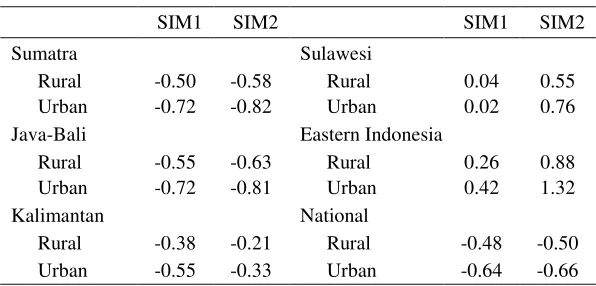
Table 5. Changes in Household Income (in %)
SIM1 SIM2 SIM1 SIM2
Sumatra Sulawesi
Rural -0.50 -0.58 Rural 0.04 0.55
Urban -0.72 -0.82 Urban 0.02 0.76
Java-Bali Eastern Indonesia
Rural -0.55 -0.63 Rural 0.26 0.88
Urban -0.72 -0.81 Urban 0.42 1.32
Kalimantan National
Rural -0.38 -0.21 Rural -0.48 -0.50
Urban -0.55 -0.33 Urban -0.64 -0.66
2009 Resosudarmo, Nurdianto & Hartono 161 every sector undergoes a contraction in both
simulations. Despite an increase in the cons-truction sectoral output, its positive impact is relatively too small to make a difference. The largest negative impact is felt by the informal professional worker in the second simulation, which is due to a large reduction in the sectoral output of other services.
3. Impacts on Household Incomes
This sub-section describes the impacts of decentralisation on household income using the two simulations mentioned above. As mentioned before, observation of household incomes is typically the ultimate observation related to observing the impacts of govern-ment policies. However, to understand what happens to household incomes due to a certain policy, one should observe the impact of that policy on labour income and sectoral perfor-mances.
From Table 6, it can be seen that all households, both rural and urban, in Sumatra, Java-Bali, and Kalimantan are negatively affected in both scenarios. Specifically, urban households are more adversely affected than rural households. This condition is caused by the fact that the largest source of household income in those three regions comes from urban manual, clerical and professional workers. For the case of Sumatra, the formal professional worker is the most negatively affected labour type, whereas for Java-Bali and Kalimantan, formal-informal professional and formal professional workers respectively are the most adversely affected labour types.
The opposite holds true for Sulawesi and Eastern Indonesia, where all households in both rural and urban areas are positively affected under both scenarios. In Sulawesi, the positive impacts on the rural and urban households are relatively small in the first simulation as only formal manual, formal clerical and professional workers receive higher incomes. Both rural and urban households in Sulawesi are more positively affected in the second simulation than in the
first due to an income increase for all labour types, bearing in mind the significant income increases to the formal manual and formal professional workers.
For the case of Eastern Indonesia, the positive impact received by the rural household in the first simulation is relatively small as almost all types of labour undergo an increase in income except for the formal-informal agricultural worker. In the meantime, the positive impacts received by both rural and urban households in the second simulation are larger than in the first simulation as there are income increases to all labour types, particularly the significant income increases to the informal clerical and formal-informal professional workers.
As for the national economy, there is an income reduction to both rural and urban households. This is due to the income reductions for all types of labour. The largest negative impact occurs to the urban household in both simulations, and far more so in the second simulation than in the first. This occurs as informal manual, formal clerical, and informal professional workers in urban areas are more negatively affected than any of the other labour types. Lastly, the negative impacts on these three labour types are greater in the second simulation than in the first.
CONCLUSIONS
Journal of Indonesian Economy and Business May 162
Second, a proportionally increased regional budget, with the consequence of a declining central government budget, does not help the economies of any region, except for that of Eastern Indonesia and it does not increase by much.
Third, if the central government cares to boost the economy of Eastern Indonesia and Sulawesi, giving significantly extra funding to these regions would work better than increasing all regional budgets proportionally. Fourth, as a consequence of the first and the third conclusions, it does not seem that reducing gaps among regional economies and boosting the national economy through a fiscal transfer strategy promote the same end. It might be an idea for the central government to concentrate a bit more of the budget at the national level than it did in 2005. However, where reducing gaps among regional econo-mies is concerned, i.e. to boost the econoecono-mies of Sulawesi and Eastern Indonesia, providing lump-sum transfers to those regions would work.
Fifth, in general, the impacts on labour income of further fiscal transfers to regions vary a great deal. However, it can be identified that in regions where informal sectors have not yet been developed, i.e. in Sumatra, Kaliman-tan, Sulawesi and Eastern Indonesia, informal labour is affected less by these policy changes than formal labour. And so transferring more funding to regions off-Java and Bali does benefit those in the formal sector more than those in the informal sector.
Sixth, in Sulawesi and Eastern Indonesia, in general, the two policies affect clerical and professional labour more than agricultural and manual workers. In this case, transferring more money to the regions (SIM2) is more beneficial for clerical and professional labour than agricultural and manual labour.
Finally, overall and on average, a more decentralised fiscal system than that of 2005 would benefit households in Sulawesi and Eastern Indonesia, as their incomes would
tend to increase. The same cannot be said for households in Java-Bali, Sumatra and Kalimantan.
REFERENCES
Alm, J., R.H. Aten, and R. Bahl, 2001. “Can
Indonesia Decentralize Successfully?
Plans, Problems, and Prospects”, Bulletin of Indonesian Economic Studies, 37(1), 83-102.
BPS or Badan Pusat Statistik [Central Statis-tical Agency] (2008), Statistical Year Book of Indonesia 2008, Jakarta: BPS. Defourny, J. and E. Thorbecke, 1984.
“Structural Path Analysis and Multiplier Decomposition Within a Social Accounting Matrix Framework”,
Economic Journal, 94(373), 111-36. Hartono, D. and B.P. Resosudarmo, 1998.
“Eksistansi matriks pengganda dan Pyatt dan Round dekomposisi dari sebuah Sistem Neraca Sosial Ekonomi [Existence of the multiplier matrix and the Pyatt and Round Decomposition Matrix for a Social
Accounting Matrix]”, Ekonomi dan
Keuangan Indonesia, 46(4), 473-496.
Pyatt, G. and J.I. Round, 1979. “Accounting
and Fixed Price Multipliers in a Social Accounting Matrix Framework”,
Economic Journal, 89, 850-73.
Reproduced in extended form as Chapter 9 of Pyatt, G. and J.I. Round (eds) (1985),
Social Accounting Matrices: A Basis for Planning, Washington, DC: The World Bank.
Sadoulet, E., and A. de Janvry, 1995.
Quantitative Development Policy Analy-sis, The Johns Hopkins, University Press.
Thorbecke, E, 1985. “The Social Accounting