de Bordeaux 16(2004), 357–371
Homology for irregular connections
parSpencer BLOCH etH´el`ene ESNAULT
R´esum´e. Nous d´efinissons sur une courbe alg´ebrique l’homologie `
a valeurs dans une connexion avec des points singuliers ´eventuelle-ment irr´eguliers, g´en´eralisant ainsi l’homologie `a valeurs dans le syst`eme local sous-jacent pour une connexion avec points sin-guliers r´esin-guliers. L’int´egration d´efinit alors un accouplement par-fait entre la cohomologie de de Rham `a valeurs dans la connexion et l’homologie `a valeurs dans la connexion duale.
Abstract. Homology with values in a connection with possibly irregular singular points on an algebraic curve is defined, gener-alizing homology with values in the underlying local system for a connection with regular singular points. Integration defines a perfect pairing between de Rham cohomology with values in the connection and homology with values in the dual connection.
0. Introduction
Consider the following formulas, culled, one may imagine, from a text-book on calculus:
√ π=
Z ∞
−∞
e−t2dt
(e2πis−1)Γ(s) = (e2πis−1)
Z ∞
0
e−ttsdt
t Gamma function
Jn(z) =
1 2πi
Z
{|u|=ǫ} exp(z
2(u− 1
u)) du
un+1 Bessel function.
theory in the irregular case. Of course, most of the “heavy lifting” was done by Malgrange op. cit. We hope, in reinterpreting his theory, to better un-derstand relations between irregular connections and wildly ramifiedℓ-adic sheaves. There are striking relations between ǫ-factors for ℓ-adic sheaves on curves over finite fields and determinants of irregular periods [8] which merit further study. Finally, relations between irregular connections and the arithmetic theory of motives remain mysterious.
LetX be a smooth, compact, connected algebraic curve (Riemann sur-face) over C. Let D = {x1, . . . , xn} ⊂ X be a non-empty, finite set of
points (which we also think of as a reduced effective divisor), and write
U := X\D֒→j X. Let E be a vector bundle on X, and suppose given a connection with meromorphic poles onD
∇:E →E⊗ω(∗D).
Here ω is the sheaf of holomorphic 1-forms on X and ∗D refers to mero-morphic poles on D. Unless otherwise indicated, we work throughout in the analytic topology. The de Rham cohomologyHDR∗ (X\D;E,∇) is the cohomology of the complex of sections
(0.1) Γ(X, E(∗D))−→∇ Γ(X, E⊗ω(∗D))
placed in degrees 0 and 1. These cohomology groups are finite dimensional [1], Proposition 6.20, (i).
LetE∨ be the dual bundle, and let∇∨ be the dual connection, so
(0.2) dhe, f∨i=h∇(e), f∨i+he,∇∨(f∨)i.
DefineE= ker(∇), andE∨ = ker(∇∨) to be the corresponding local systems of flat sections onU. We want to define homology with values in these local systems, or more precisely with values in associated cosheaves on X. For
x∈X\D,Ex will denote the stalk ofE atx. Define the co-stalk at 0∈D
(0.3) E0 :=Ex/(1−σ)Ex
wherex6= 0 is a nearby point, andσ is the local monodromy about 0. We write Cn =Cn(E,∇) for the group of n-chains with values in E and rapid
decay near 0. Write ∆n for the n-simplex and b∈ ∆n for its barycenter. Thus,Cn(E,∇) is spanned by elementsc⊗ǫwithc: ∆n→X andǫ∈ Ec(b),
whereb∈∆n is the barycenter. We assume c−1(0) = union of faces⊂∆n and thatǫ hasrapid decay nearD. This is no condition if D∩c(∆n) =∅.
If 0∈D∩c(∆n), we takeei a basis for E near 0 and write ǫ=Pfic∗(ei).
There is a natural boundary map
(0.4) ∂:Cn(E,∇)→ Cn−1(E,∇); ∂(c⊗ǫ) = X
(−1)jcj⊗ǫj
where cj are the faces of c. Note if bj is the barycenter of the j-th face
and c(bj) 6= 0, c determines a path from c(b) to c(bj) which is canonical
upto homotopy on ∆\ {0}. (As a representative, one can take c[bj, b], the
image of the straight line frombtobj. By assumption,c−1(0) is a union of
faces, so it does not meet the line.) Thus ǫ∈ Ec(b) determines ǫj ∈ Ec(bj).
Similarly for 0∈D, ifc(bj) = 0 there is corresponding toǫa uniqueǫj ∈ E0
because we have taken coinvariants. If c: ∆n→ D is a constant simplex, there is no rapid decay condition.
It is straightforward to compute that∂◦∂= 0. Considerc⊗ǫ. Ifc(b) = 0, whereb∈∆2 is the barycentre, thenc(∆2) = 0 andǫ=ǫi = (ǫi)j ∈ E0 for
alliandj involved, thus the condition is trivially fulfilled. If not, and some
c(bi) = 0, then (ǫj)i= (ǫi)j ∈ E0 for allj, and if allc(bi)6= 0, then one has
by unique analytic continuation inc(∆2) the relation (ǫi)j = (ǫj)i ∈ Eedgeij
for all i, j, if edgeij 6= 0, else in E0.
We define
(0.5) H∗(X, D;E∨,∇∨) :=H∗
C∗(X;E∨,∇∨)/C∗(D;E∨,∇∨)
.
(The growth condition means this depends on more than just the topo-logical sheafE∨, so we keep E∨,∇∨ in the notation.)
We now define a pairing
( , ) :HDR∗ (X\D;E,∇)×H∗(X, D;E∨,∇∨)→C; ∗= 0,1 (0.6)
by integrating over chains in the following manner. For ∗ = 0, then
H0(X, D;E∨,∇∨) is generated by sections of the dual local system E∨ in
points∈X whileHDR0 (X\D;E,∇) is generated by global flat sections in
E with moderate growth. So one can pair them. For ∗ = 1, since D6= ∅, then
HDR1 (X\D;E,∇) =H0(X, ω⊗E(∗D))/∇H0(X, E(∗D)),
and since classes c⊗ǫgenerating H0(X, D;E∨,∇∨) have rapid decay, the
integralRc< fic∗(ei), α >is convergent, whereα∈H0(X, ω⊗E(∗D)) and < >is the duality betweenE∨ and E.
The rest of the note is devoted to the proof of the following theorem.
Theorem 0.1. The process of integrating forms over chains is compati-ble with homological and cohomological equivalences and defines a perfect pairing of finite dimensional vector complex spaces
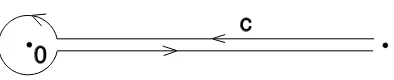
0
c
Figure 1. c⊗e−tts represents a class in H 1
Example 0.2. (i). If ∇has regular singular points, there are no rapidly decaying flat sections, so H∗(X, D;E∨,∇∨) ∼= H∗(X \ D;E∨). Also,
HDR∗ (X\D;E,∇) ∼= H∗(U,E) (cf. [1], Th´eor`eme 6.2), and the theorem becomes the classical duality between homology and cohomology.
(ii). Suppose X = P1, D = {0,∞}. Let E = OP1 with connection
∇(1) = −dt+sdtt, for some s ∈ C\ {0,1,2, . . .}. Then E ⊂ EU = OU
is the trivial local system spanned byett−s, so E∨ ⊂E∨
U =OU is spanned
bye−tts. We consider the pairingHDR1 ×H1→Cfrom theorem 0.1. Note
first thatHDR1 has dimension 1, spanned by dtt. This can either be checked directly from (0.1), using
∇(tp) = ((p+s)tp−1−tp)dt,
or by showing the de Rham cohomology is isomorphic to the hypercoho-mology of the complexOP1 →∇ ω((0) + 2(∞)), which is easily computed. To computeH1(X, D;E∨,∇∨), the singularity at 0 is regular, so there are no
non-constant, rapidly decaying chains at 0. The section ǫ∨ := e−tts of E∨ is rapidly decaying on the positive real axis near∞, so the chain c⊗ǫ∨ in fig. 1 above represents a 1-cycle. We have
(c⊗e−tts,dt t ) = (e
2πis−1)Z ∞
0
e−ttsdt t
which is a variant of Hankel’s formula (see [10], p. 245).
(iii). Let X, D, E be as in (ii), but take ∇(1) = 12(d(zu)−d(uz)) for some
z ∈ C\ {0}. Here the connection has pole order 2 at 0 and ∞ and it has trivial monodromy. Arguing as above, one computes dimHDR1 = 2, generated by updu, p ∈ Z, with relations updu = −2p
zup−1du−up−2du.
The Gauß-Manin connection on this group is
∇GM(updu) =
1 2(u
p+1−up−1)du∧dz.
Assume Im(z) >0. Then the vector space H1(P1,{0,∞};E∨,∇∨) is
gen-erated by
{|u|= 1} ⊗exp(1 2z(u−
1
u)), and [0, i∞]⊗exp(
1 2z(u−
1
(If Im(z)6>0, then the second path must be modified.) The integrals
are periods and satisfy the Bessel differential equation
z2d
The functionJn is entire. To show thatHn is linearly independent of Jn,
it will then be sufficient to show that Hn is unbounded on the positive
part of the imaginary axis Re(z) = 0 as z → 0. Making the coordinate
1 , and making the change of variable v→ 1v in the integral R1
where in the last inequality, we have assumed that 2y ≤ 1. This last integral is, up to something bounded, equal to 2R2y1 dvv =−2 log(2y), which is unbounded, asy >0, y→0.
Usually, for integers n∈ Z, one considers Jn as one standard solution,
but notHn(see [10], p.371). Finally, to get Bessel functions for non-integral
1. Chains
Let D={x1, . . . , xn} be as above, and let ∆i be a small disk about xi
for each i. Letδi be the boundary circle. Define
(1.1) H∗(∆i, δi∪ {xi};E,∇)
=H∗
C∗(∆i;E,∇)/(C∗(δi;E,∇) +C∗({xi};E,∇)
(Note, for a set like δi which is closed and disjoint from D, our chains
coincide with the usual topological chains with values in the local system
E. The groupC∗({xi};E,∇) consists of constant chainsc: ∆n→ {xi}with
values in
Exi :=Ex/(1−µi)Ex
for somexnearxi as in (0.3), whereµi is the local monodromy aroundxi.)
In the following theorem,H∗(U,E) is the standard homology associated to the local system on U =X\D.
Theorem 1.1. With notation as above, there is a long exact sequence
(1.2) 0→H1(U,E)→H1(X, D;E,∇)→ ⊕iH1(∆i, δi∪ {xi};E,∇) →H0(U,E)→H0(X, D;E,∇)→0.
Proof. Let C∗ := C∗(X;E,∇)/C∗(D;E,∇) be the complex calculating
H∗(X, D;E,∇), and let
C∗(U)⊂ C∗
be the subcomplex calculating H∗(U,E), i.e. the subcomplex of chains whose support is disjoint from D. Of course, one has C∗(U;E,∇) =
C∗(U;E), which justifies the notation.
WriteB=C∗/C∗(U). There is an evident map of complexes
(1.3) ψ:⊕iC∗(∆i, δi∪ {xi};E,∇)→ B
which must be shown to be a quasi-isomorphism. Let
B(i) =ψ(C∗(∆i, δi∪ {xi};E,∇)) = C∗(∆i, δi∪ {xi};E,∇)/C∗(∆i\ {xi};E)⊂ B.
Obviously the map α:⊕iB(i) ֒→ B is an inclusion. We claim first that α
is a quasi-isomorphism. To see this, note that all these complexes admit subdivision maps subd which are homotopic to the identity. Given a chain
c ∈ B, there exists an N such that subdN(c) ∈ ⊕B(i). Taking c with
It remains to show the surjective map of complexes
β:C∗(∆i, δi∪ {xi};E,∇)→ B(i)
is a quasi-isomorphism. The kernel ofβ is
C∗(∆i\ {xi};E)/C∗(δi;E),
which is acyclic asδi֒→∆i\ {xi}admits an evident homotopy retract.
The next point is to show
(1.4) H∗(∆i, δi∪ {xi};E,∇) = (0); i= 0,2.
The assertion forH0is easy because any pointyin ∆i\{xi}can be attached
to δi by a radial path r not passing through xi. Then ǫ ∈ Ey extends
uniquely to ǫ on r and ∂(r⊗ǫ) ≡ y⊗ǫ mod chains onδi. Vanishing in
(1.4) wheni= 2 will be proved in a sequence of lemmas. For convenience we drop the subscripti and replacexi with 0.
Lemma 1.2. Let ℓ⊂∆be a radial line meeting δ atp. LetEℓ be the space
of sections of the local system along ℓ\ {0} with rapid decay at 0. Then
H∗(ℓ,{0, p};E,∇)∼=
(
0 ∗ 6= 0
Eℓ ∗= 1.
Proof of lemma. LetC∗(ℓ) be the complex of chains calculating this homol-ogy, and letC∗(ℓ\ {0})⊂ C∗(ℓ) be the subcomplex of chains not meeting 0. ThenC∗(ℓ\ {0}) is contractible, and
C∗(ℓ)/C∗(ℓ\ {0})= (C∼ ∗(ℓ)/C∗(ℓ\ {0}))⊗ Eℓ
whereC∗ denotes classical topological chains. The result follows. One knows from the theory of irregular connections in dim 1 [4] that ∆\ {0} can be covered by open sectorsV (∆ such than
(1.5) E,∇|V ∼=⊕i(Li⊗Mi)
whereLi is rank 1 andMi has a regular singular point. LetW ⊂V ∪ {0}
be a smaller closed sector with outer boundary δW = δ∩W and radial
sides ℓ1, ℓ2. Recall the Stokes lines are radial lines where the horizontal
sections of the Li shift from rapid decay to rapid growth. We assume W contains at most one Stokes line, and that ℓ1, ℓ2 are not Stokes lines.
WritingW =W1∪W2, where Wi are even smaller sectors, each of which
containing the Stokes line if there is one, one may think of the following lemma as a Mayer-Vietoris sequence.
Lemma 1.3. With notation as above, let w be a basepoint in the interior of W. Then
H∗(W, δW ∪ {0};E,∇)∼= (
0 ∗ 6= 1
Proof of lemma. One has
⊕iH1(ℓi,{0, pi};E,∇)→H1(W, δW ∪ {0};E,∇)
and of course the assertion of the lemma is that this coincides with Eℓ1 ⊕
Eℓ2 → Eℓ1+Eℓ2. To check this, by (1.5) one is reduced to the caseE=L⊗M whereL has rank 1 andM has regular singular points.
IfW does not contain a Stokes line forLthenEℓ1 =Eℓ2 =Eℓ1+Eℓ2, and the argument is exactly as in lemma 1.2.
Suppose W contains a Stokes line for L. Then (say) Eℓ1 = Ew and
Eℓ2 = (0). Let C∗(W) be the complex of chains calculating the desired homology, and letC∗(W \ {0}) ⊂ C∗(W) be the chains not meeting 0. As in the previous lemma,C∗(W \ {0}) is acyclic. We claim the map
C∗(ℓ1)→ C∗(W)/C∗(W \ {0})
is a quasi-isomorphism. If we choose an angular coordinateθ such that
ℓ1 :θ= 0; Stokes :θ=a >0; ℓ2 :θ=b > a,
then rotation reiθ 7→ re(1−t)iθ provides a homotopy contraction of the in-clusion ofℓ1 ⊂W. This homotopy contraction preserves the condition of
rapid decay, proving the lemma.
Letπd: ∆→∆ be the ramified cover of degreedobtained by taking the d-th root of a parameter at 0. By the theory of formal connections [4], one has, for suitable d, a decomposition as in (1.5) for the formal completion of the pullbackπd∗
dE ∼=⊕iLi⊗Mi. Letmi be the degree of the pole of the
connection onLiwhen we identifyLi ∼=Ob, i.e. ∇Li(1) =gi(z)dzfor a local
parameterz, and mi is the order of pole of gi.
Lemma 1.4. We have
dimHp(∆, δ∪ {0};E,∇) = (
0 p6= 1
1 d
P
mi≥2(mi−1) dim(Mi) p= 1.
Proof of lemma. Assume first that we have a decomposition of the type (1.5) on Eb itself, i.e. that no pullback π∗d is necessary. We write ∆ as a union of closed sectorsW0, . . . , WN−1 where Wi has radial boundary lines ℓiandℓi+1. We assume eachWihas at most one Stokes line. Using excision
together with the previous lemmas we get
(1.6) 0→H2(∆, δ∪ {0};E,∇)→ ⊕i=0N−1H1(ℓi,{pi,0};E,∇) ν
→ ⊕Ni=0−1H1(Wi, δWi∪ {0};E,∇)→H1(∆, δ∪ {0};E,∇)→0.
By lemma 1.3, the map ν above is given by
An element in the kernel ofν is thus a sectioneofE|∆−{0} which has rapid decay along eachℓi. Since each Wi contains at most one Stokes line, such
anewould necessarily have rapid decay on every sector and thus would be trivial. This proves vanishing forH2(∆, δ;E,∇). Finally, to compute the
dimension of H1, note that if Li has a connection with pole of order mi,
then it has a horizontal section of the formef, wheref has a pole of order mi −1. (The connection is 1 7→ df.) Suppose f = az1−mi+. . .. Stokes
lines for this factor are radial lines where az1−mi is pure imaginary. Thus,
there are 2(mi−1) Stokes lines for this factor. Consider one of the Stokes
lines, and suppose it lies in Wk. If the real part of az1−mi changes from
negative to positive as we rotate clockwise through this line, say we are in case +, otherwise we are in case−. We have
(1.7) dim(Eℓk+Eℓk+1)−dimEℓk =
(
0 case + dim(Mi) case −,
since the two cases alternate, we get a contribution of (mi−1) dim(Mi). If mi ≤1 there are no rapidly decaying sections, so that case can be ignored.
Summing over iwithmi ≥2 gives the desired result.
Finally, we must consider the general case when the decomposition (1.5) is only available on πd∗
dE for some d≥2. By a trace argument, vanishing
of the homology upstairs, i.e. for πd∗
dE, in degrees 6= 1 implies vanishing
downstairs. Since πd : ∆\ {0} → ∆\ {0} is unramified, an Euler
charac-teristic argument (or, more concretely, just cutting into small sectors over which the covering splits) shows that the Euler characteristic multiplies by
dunder pullback, proving the lemma.
In particular, we have now completed the proof of theorem 1.1.
2. de Rham Cohomology
In this section, using differential forms, we construct the dual sequence to the homology sequence from theorem 1.1. (More precisely, we continue to work withE,∇, so the sequence we construct will be dual to the homology sequence with coefficients inE∨,∇∨). Consider the diagram of complexes
(2.1)
0 −→ E(∗D) −→ j∗EU −→ j∗EU/E(∗D) −→ 0
∇mero
y ∇an
y ∇an/mero
y
0 −→ E(∗D)⊗ω −→ j∗EU⊗ω −→ (j∗EU/E(∗D))⊗ω −→ 0.
A result of Malgrange [6] is that∇an/merois surjective. DefineN :=⊕iNi =
and applying the serpent lemma:
(2.2) 0→HDR0 (U;E,∇)→H0(U,E)→N
→HDR1 (U;E,∇)→H1(U,E)→0.
Theorem 2.1. Integration of forms over chains defines a perfect pairing between the exact sequence (2.2)and the exact sequence from theorem 1.1:
(2.3) 0→H1(U,E∨)→H1(X, D;E∨,∇∨)→ ⊕iH1(∆i, δi∪ {xi};E∨,∇∨) →H0(U,E∨)→H0(X, D;E∨,∇∨)→0.
Proof. To establish the existence of a pairing, note that if c⊗ǫ∨ is a rapidly decaying chain and η is a form of the same degree with mod-erate growth, then elementary estimates show Rchǫ∨, ηi is well defined. Suppose c : ∆n → X and write ∆n = lim
t→0∆nt where ∆nt denotes
∆n\tubular neighborhood of radiust around∂∆n. Letct=c|∆n
t and
sup-pose η=dτ whereτ has moderate growth also. Then
(2.4)
Note ∂c may include simplices mapping to D. Our definition (0.5) of
C∗(X, D;E∨,∇∨) factors these chains out. Thus, we do get a pairing of complexes.
Of course, chains away fromDintegrate with forms with possible essen-tial singularities onD. To complete the description of the pairing, we must indicate a pairing
(2.5) ( , ) :Ni×H1(∆i, δi∪ {xi};E∨,∇∨)→C.
To simplify notation we will drop the subscript i and take xi = 0. An
element in H1 can be represented in the form ǫ∨ ⊗c where c is a radial
path. Let c∩δ = {p}. Given n∈ N, choose a sector W containing c on which E has a basis ǫi. By assumption, we can representn=Paiǫi with ai analytic on the open sector, such that
(2.6) ∇(Xaiǫi) = X
ǫi⊗dai= X
ei⊗ηi
whereei from a basis ofE in a neighborhood of 0 and ηi are meromorphic
1-forms at 0. then by definition
(2.7) (ǫ∨⊗c, n) :=
p top′. Then Cauchy’s theorem (together with a limiting argument at 0)
Similar arguments show the pairing independent of the choice of the radius of the disk. Also, if Paiǫi =Pbiei withbi meromorphic at 0, then
It follows that the pairing is well defined.
Lemma 2.2. The diagrams
Proof of lemma. Consider the top square. The top arrow is excision, re-placing a chain with the part of it lying in the disks ∆i. The bottom arrow
maps annas above in someNi toPej⊗ηj =Pǫj⊗daj. Alongcoutside
the disksPej⊗ηj is exact; its integral along the chain is a sum of terms of
the formPihǫ∨, ǫjiaj(pi) wherepi ∈c∩δi. For the part of the chain inside
the ∆i of course we must takeRc∩∆ihǫ∨, ejiηj. Combining these terms with
appropriate signs yields the desired compatibility.
section ǫ on U the corresponding element in N. Note here the aj will be
constant so in the pairing withN only the term −Phǫ∨, ǫjiaj(p) survives.
The assertion of the lemma follows.
Returning to the proof of the theorem, we see it reduces to a purely local statement for a connection on a disk. In the following lemma, we modify notation, writingN to denote the corresponding group for a connection on a disk ∆ with a meromorphic singularity at 0.
Lemma 2.3. The pairing
( , ) :N ×H1(∆, δ;E∨,∇∨)→C
is nondegenerate on the left, i.e. (ǫ∨ ⊗c, n) = 0 for all relative 1-cycles implies n= 0.
Proof of lemma. We work in a sector and we suppose the basis ǫi taken
in the usual way compatible (in the sector) with the decomposition into a direct sum of rank 1 irregular connections tensor regular singular point connections. Let ǫ∨i be the dual basis.
Fix an i and suppose first ǫi and ǫ∨i both have moderate growth. We
claimai has moderate growth. For this it suffices to showdaihas moderate
growth. But
(2.10) dai =h∇(n), ǫ∨ii= X
j
hej, ǫ∨iiηj.
This has moderate growth because,ej, ǫ∨i,and ηj all do.
Now assume (ǫ∨⊗c, n) = 0 for all ǫ∨ ⊗c ∈ H1. Fix an i and assume ǫ∨
i is rapidly decreasing in our sector. Let c be a radius in the sector with
endpointp. We can find (cf. [4], chap. IV, p.53-56) a basis ti of E on the
sector with moderate growth and such thatti =ψiǫi, sot∨i =ψi−1ǫ∨i.
We are interested in the growth ofaiǫi along c. We have
(2.11)
ai(p)ǫi(p) = Z
c X
j
hǫ∨i , ejiηj
ǫi(p) = Z
c ψi
X
j
ht∨i , ejiηj
ψi(p)−1ti(p).
Asymptotically, taking y the parameter along c, ψi(y) ∼ exp(−ky−N) as y→0 for somek >0 and some N ≥1. We need to know the integral
(2.12) exp(kp−N)
Z p
0
has moderate growth as p → 0. Changing variables, so x = y−1, q = p−1, u=x−q, this becomes
(2.13)
Z ∞
0
(u+q)M−2exp(qN −(u+q)N)du
=
Z ∞
0
(u+q)M−2exp(−uN −qf(u, q))du,
wheref is a sum of monomials inq anduwith positive coefficients. Clearly this has at worst polynomial growth asq→ ∞ as desired.
Finally, assumeǫ∨i is rapidly increasing andǫi is rapidly decreasing. We
have as above
(2.14) X
i
ej⊗ηj = X
j
ǫj⊗daj = X
j
ψj−1tj ⊗daj.
In particular, ψi−1dai has moderate growth. This implies aiǫi = aiψ−i 1ti
has moderate growth as well. Indeed, changing notation, this amounts to the assertion that ifg is rapidly decreasing and gdzdf has moderate growth, thengf has moderate growth. Fix a point p0 with 0< p < p0. the mean
value theorem says there exists anr with p≤r≤p0 such that
g(p)f(p) =g(p)(f(p0) + (p−p0)f′(r)).
Suppose|f′(q)g(q)|<< q−N. We get
|g(p)f(p)|<<|g(p)f′(r)| ≤ |g(r)f′(r)|<< r−N ≤p−N
proving moderate growth.
We conclude that our representation for n has moderate growth, and hence it is zero inN. It follows that the pairingN×H1 →Cis
nondegen-erate on the left.
Returning to the global situation, we have now
dimNi≤dimH1(∆i, δi;E∨,∇∨),
and to finish the proof of the theorem, it will suffice to show these dimen-sions are equal.
Lemma 2.4. With notation as above, dimNi= dimH1(∆i, δi;E∨,∇∨).
Proof of lemma. It will suffice to compute the difference of the two Euler characteristics
(2.15) χ(U,E)−χDR(U;E,∇).
E⊗Kbxi ∼=⊕jLij⊗Mij withLij rank 1 andMij at worst regular singular.
(HereKbxi is the Laurent power series field atxi). Letmij be the degree of
the pole for the connection onLij. Then one can find coherent sheaves
F2⊂F1 ⊂E(∗D)
such that
F1/F2 ∼=⊕ijMij/Mij(−mijxi),
E∇⊂H0(F2);∇(F2)⊂F1⊗ω,
H0(F1⊗ω)։HDR1 (U;E,∇).
It follows that, writing g= genus(X),
(2.16) χDR(U;E,∇)
=χ(F2)−χ(F1⊗ω) =−rk(E)(2g−2)− X
ij
mijdim(Mij).
Since
(2.17) χ(U,E) =−rk(E)(2g−2 +n),
(which is proven algebraically as above, replacing∇by the regular connec-tion associated toE) it follows that
χDR(U;E,∇)−χ(U,E) =− X
ij
(mij −1) dim(Mij).
Referring to lemma 1.4, we see that this is the desired formula.
This completes the proof of the theorem.
References
[1] P. Deligne,Equations Diff´´ erentielles `a Points Singuliers R´eguliers. Lecture Notes in Math-ematics163, Springer Verlag, 1970.
[2] N. Kachi, K. Matsumoro, M. Mihara,The perfectness of the intersection pairings for
twisted cohomology and homology groups with respect to rational1-forms. Kyushu J. Math.
53(1999), 163–188.
[3] G. Laumon,Transformation de Fourier, constantes d’´equations fonctionnelles, et
conjec-ture de Weil. Publ. Math. IHES65(1987), 131–210.
[4] B. Malgrange,Equations Diff´´ erentielles `a Coefficients Polynomiaux. Progress in Math.
96, Birkh¨auser Verlag, 1991.
[5] B. Malgrange,Remarques sur les ´equations diff´erentielles `a points singuliers irr´eguliers. Springer Lecture Notes in Mathematics712(1979), 77–86.
[6] B. Malgrange, Sur les points singuliers des ´equations diff´erentielles. L’Enseignement math´ematique, t.20, 1-2(1974), 147–176.
[7] T. Saito, T. Terasoma,Determinant of Period Integrals. J. AMS10(1997), 865–937. [8] T. Terasoma,Confluent Hypergeometric Functions and Wild Ramification. Journ. of
Al-gebra185(1996), 1–18.
[9] T. Terasoma, A Product Formula for Period Integrals. Math. Ann.298(1994), 577–589. [10] G.N. Watson, E.T. Whittaker, A Course of modern Analysis. Cambridge University
SpencerBloch Dept. of Mathematics University of Chicago Chicago, IL 60637, USA
E-mail:[email protected]
H´el`eneEsnault Mathematik Universit¨at Essen FB6, Mathematik 45117 Essen, Germany