ELECTRONIC COMMUNICATIONS in PROBABILITY
MAXIMUM OF DYSON BROWNIAN MOTION AND NON-COLLIDING
SYSTEMS WITH A BOUNDARY
ALEXEI BORODIN1
Mathematics Department, California Institute of Technology, Pasadena, CA 91125, USA email: [email protected]
PATRIK L. FERRARI
Institut für Angewandte Mathematik, Abt. Angewandte Stochastik, Endenicher Allee 60, Universität Bonn, 53115 Bonn, Germany
email: [email protected]
MICHAEL PRÄHOFER
Zentrum Mathematik, Bereich M5, Technische Universität München, D-85747 Garching bei München, Deutschland
email: [email protected]
TOMOHIRO SASAMOTO2
Department of Mathematics and Informatics, Chiba University, 1-33 Yayoi-cho, Inage, Chiba 263-8522, Japan
email: [email protected]
JON WARREN
Department of Statistics, University of Warwick, Coventry, CV4 7AL, UK email: [email protected]
SubmittedJune 2, 2009, accepted in final formOctober 16, 2009 AMS 2000 Subject classification: 60K35, 60J65, 60J55
Keywords: Dyson Brownian motion, reflected Brownian motion, non-colliding systems with a wall
Abstract
We prove an equality-in-law relating the maximum of GUE Dyson’s Brownian motion and the non-colliding systems with a wall. This generalizes the well known relation between the maximum of a Brownian motion and a reflected Brownian motion.
1PARTIALLY SUPPORTED BY NSF GRANT DMS-0707163.
2PARTIALLY SUPPORTED BY THE GRANT-IN-AID FOR YOUNG SCIENTISTS (B), THE MINISTRY OF EDUCATION,
CUL-TURE, SPORTS, SCIENCE AND TECHNOLOGY, JAPAN.
1
Introduction and Results
Dyson’s Brownian motion model of GUE (Gaussian unitary ensemble) is a stochastic process of po-sitions ofmparticles,X(t) = (X1(t), . . . ,Xm(t))described by the stochastic differential equation,
d Xi=d Bi+
whereBi, 1≤i≤mare independent one dimensional Brownian motions[6]. The process satisfies
X1(t)<X2(t)<· · ·<Xm(t)for allt>0. We remark that the processX can be started from the
origin, i.e., one can takeXi(0) =0, 1≤i≤m. See[11].
One can introduce similar non-colliding system ofmparticles with a wall at the origin[8, 9, 17]. The dynamics of the positions of the mparticles X(C) = (X(C)
This process is referred to as Dyson’s Brownian motion of typeC. It can be interpreted as a system ofmBrownian particles conditioned to never collide with each other or the wall.
One can also consider the case where the wall above is replaced by a reflecting wall[9]. The dynamics of the positions of themparticlesX(D)= (X1(D), . . . ,Xm(D))satisfying 0≤X1(t)<X2(t)<
· · ·<Xm(t)for allt>0, is described by the stochastic differential equation,
d Xi(D)=d Bi+1
where L(t) denotes the local time of X1(D) at the origin. This process will be referred to as Dyson’s Brownian motion of type D. Some authors consider a process defined by the s.d.e.s (1.3) without the local time term. In this case the first component of the process is not con-strained to remain non-negative, and the process takes values in the Weyl chamber of type D, {|x1|< x2< x3. . .< xm}. The process we consider with a reflecting wall is obtained from this
by replacing the first component with its absolute value, with the local time term appearing as a consequence of Tanaka’s formula.
It is known the processesX(C)andX(D)can be obtained using the Doobh-transform, see[8, 9]. Let(Pt0,(C);t≥0), resp. (Pt0,(D);t≥0), be the transition semigroup formindependent Brownian motions killed on exiting{0<x1<x2. . .<xm}, resp. the transition semigroup formindependent Brownian motions reflected at the origin killed on exiting{0≤x1<x2. . .<xm}. From the Karlin-McGregor formula, the corresponding densities can be written as
det{φt(xi−x′j)−φt(xi+x′j)}1≤i,j≤m, (1.4) resp.,
whereφt(z) = p1
For notational simplicity we suppress the indexC,Dfor the semigroups and inhin the following. Then one can show that h(x)is invariant for the Pt0 semigroup and we may define a Markov semigroup by
Pt(x,d x′) =h(x′)Pt0(x,d x′)/h(x). (1.7) This is the semigroup of the Dyson non-colliding system of Brownian motions of type C andD. Similarly to theX process, the processesX(C)andX(D)can also be started from the origin (see[4] or use Lemma 4 in[9]and apply the same arguments as in[11]).
In GUE Dyson’s Brownian motion of nparticles, let us take the initial conditions to be Xi(0) =
0, 1≤i≤n. The quantity we are interested in is the maximum of the position of the top particle for a finite duration of time, max0≤s≤tXn(s). In the sequel we write sup instead of max to conform
with common usage in the literature. Letmbe the integer such thatn=2mwhennis even and n=2m−1 whennis odd. Consider the non-colliding systems ofX(C), resp. X(D), ofmparticles starting from the origin,X(iC)(0) =0, 1≤i≤m, resp.X(iD)(0) =0, 1≤i≤m.
Our main result of this note is
Theorem 1. Let X and X(C),X(D)start from the origin. Then for each fixed t
means the Skorokhod construction to pushZj+1up fromZj. More precisely,
Z1(t) =B1(t),
Zj(t) = sup
0≤s≤t
(Zj−1(s) +Bj(t)−Bj(s)), 2≤ j≤n, (1.9)
whereBi, 1≤i≤nare independent Brownian motions, each starting from 0. The process is the
same as the process(X1 1(t),X
now a Brownian motion reflected at the origin (again by Skorokhod construction). Similarly to (1.9), From the results in[11, 5, 18], we know
and hence
sup
0≤s≤t
Xn(s)=d sup
0≤s≤t
Zn(s). (1.12)
In this note we show
Proposition 2. The following equalities in law hold between processes: (Y2m(t);t≥0)= (Xd (C)
m (t);t≥0),
(Y2m−1(t);t≥0)= (Xd (D)
m (t);t≥0),
(1.13)
m∈N.
The proof of this proposition is given in Section 2. The idea behind it is that the processes(Yi)i≥1,
(X(jC))j≥1and(X(jD))j≥1could be realized on a common probability space consisting of Brownian motions satisfying certain interlacing conditions with a boundary [18, 19]. Such a system is expected to appear as a scaling limit of the discrete processes considered in [3, 19]. In this enlarged process, the processes Yn(t) and X(C)
m (t)or X
(D)
m (t)just represent two different ways
of looking at the evolution of a specific particle and so the statement of Proposition 2 follows immediately. Justification of such an approach is however quite involved, and we prefer to give a simple independent proof. See also[5]for another representation ofXm(C)andXm(D)in terms of independent Brownian motions.
Then to prove (1.8) it is enough to show
Proposition 3. For each fixed t we have sup
0≤s≤t
Zn(s) d
=Yn(t). (1.14)
This is shown in Section 3. Forn=1 case, this is well known from the Skorokhod construction of reflected Brownian motion[12]. Then>1 case can also be understood graphically by reversing time direction and the order of particles. This relation could also be established as a limiting case of the last passage percolation. In fact the identities in our theorem was first anticipated from the consideration of a diffusion scaling limit of the totally asymmetric exclusion process with 2 speeds [1](in particular the last part of sections 1,2 and section 7).
Before closing the section, we remark that similar maximization properties of Dyson’s Brownian motion have been considered for other boundary conditions in[15, 10, 7].
Acknowledgments.
TS thanks S. Grosskinsky and O. Zaboronski for inviting him to a workshop at University of War-wick, and N. O’Connell and H. Spohn for useful discussions and suggestions.
2
Proof of Proposition 2
Lemma 4. Suppose that{X(t):t≥0}is a Markov process with state space E, evolving according to a transition semigroup(Pt;t≥0)and with initial distributionµ. Suppose that{Y(t):t≥0}is a Markov process with state space F , evolving according to a transition semigroup(Qt;t≥0)and with initial distribution ν. Suppose further that L is a Markov transition kernel from E to F , such that
µL=νand the intertwining PtL= LQt holds. Now let f :E→ G and g:F →G be maps into a third state space G, and suppose that
L(x,·)is carried by{y∈F:g(y) = f(x)}for each x∈E. Then we have
{f(X(t)):t≥0}=d {g(Y(t)):t≥0}, in the sense of finite dimensional distributions.
Proof of Lemma 4. For any bounded functionαonGletΓ1α be the functionα◦f defined on E
and letΓ2αbe the functionα◦gdefined onF. Then it follows from the condition thatL(x,·)is carried by{y∈F :g(y) =f(x)}that wheneverhis a bounded function defined onF then
L(Γ2α×h) = Γ1α×Lh, (2.1)
which is shorthand for R L(x,d y)Γ2α(y)h(y) = Γ1α× Lh. For any bounded test functions
α0,α1,· · ·,αndefined onG, and times 0< t1<· · ·< tn, we have, using the previous equation
and the intertwining relation repeatedly,
E[α0(g(Y(0)))α1(g(Y(t1))). . .αn(g(Y(tn)))] =ν(Γ2α0×Qt1(Γ2α1×Qt2−t1(· · ·(Γ2αn−1×Qtn−tn
−1Γ2αn)· · ·)))
=µL(Γ2α0×Qt1(Γ2α1×Qt2−t1(· · ·(Γ2αn−1×Qtn−tn−1Γ2αn)· · ·)))
=µ(Γ1α0×Pt1(Γ1α1×Pt2−t1(· · ·(Γ1αn−1×Ptn−tn−1Γ1αn)· · ·)))
=E[α
0(f(X(0)))α1(f(X(t1))). . .αn(f(X(tn)))] (2.2)
which proves the equality in law.
We let (Y(t): t≥ 0)be the processY ofn reflected Brownian motions with a wall introduced in the previous section. It is clear from the construction (1.10) that the process Y is a time homogeneous Markov process. We denote its transition semigroup by Qt;t ≥0). It turns out
that there is an explicit formula for the corresponding densities. Recallφt(z) =p2πt1 e−z
2/(2t)
. Let us defineφ(tk)(y) = dk
d ykφt(y)fork≥0 andφ
(−k)
t (y) = (−1)k
R∞
y
(z−y)k−1
(k−1)! φt(z)dzfork≥1.
Proposition 5. The transition densities qt(y,y′)from y= (y1, . . . ,yn)at t=0to y′= (y1′, . . . ,yn′)
at t of the Y process can be written as
qt(y,y′) =det{ai,j(yi,y′j)}1≤i,j≤n (2.3) where ai,jis given by
ai,j(y,y′) = (−1)i−1φ
(j−i)
t (y+y′) + (−1)i+jφ
(j−i)
t (y−y′). (2.4)
z1
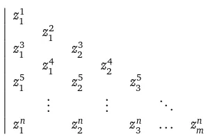
Figure 1: The setK. The triangle represents the intertwining relations of the variablesz and the vertical line on the left indicatesz12k+1≥0, see (2.5),(2.6). The set of variables on the bottom line is denoted byb(z)and the one on the upper right line bye(z).
Proof of Proposition 5.For a fixed y′, defineG(y,t)to be (2.3) as a function of yandt. We check thatGsatisfies (i) the heat equation, (ii) the boundary conditions ∂G
∂y1|y1=0=0,
∂G
∂yi|yi=yi−1=0, i=
2, 3, . . . ,nand (iii) the initial conditionsG(y,t=0) =Qin=1δ(yi−yi′).
(i) holds since φ(tk)(y) for each k satisfies the heat equation. (ii) follows from the relations,
∂ remaining part is shown in Lemma 7 in[18].
Forn=2m, resp. n=2m−1 we take(X(t),t≥0)to be Dyson Brownian motion of typeC, resp. of typeD. The transition semigroup Pt;t≥0
of this process is given by (1.7). LetKdenote the set withnlayersz= (z1,z2, . . . ,zn)wherez2k= (z2k
The kernelL0is defined by
L0g(x) =
where the integrals are taken with respect to Lebesgue measure but integrations with respect toz on the RHS is forb(z) =x fixed.
The functionhdefined at (1.6) is equal to the Euclidean volume ofK(x). Consequently we may defineLto be the Markov kernel L(x,d y) =L0(x,d y)/h(x). In the remaining part of this section
we show
Proposition 6.
Now if we apply Lemma 4 with f(x) =xm,g(y) = ynand the initial conditions starting from the origin we obtain (1.13).
Proof of Proposition 6.The kernelsPt(x,·)andL(x,·)are continuous inx. Thus we may consider x in the interior ofE, and it is enough to prove
(L0Q
t)(x,d y) = (Pt0L
0)(x,d y). (2.9)
From the definition of the kernelL0, this is equivalent to showing
Z
K(x)
qt(e(z),y)dz=
Z
K[y]
p0t(x,b(z))dz (2.10)
whereqt andp0are densities corresponding toQ
t andPt0. Integrations with respect toz are on
the LHS withb(z) =xfixed and on the RHS withe(z) =yfixed.
Let us consider the case where n= 2m. Using the determinantal expressions forqt and p0 t we
show that both sides of (2.10) are equal to the determinant of size 2mwhose(i,j)matrix element isa2i,j(0,yj)for 1≤i≤m, 1≤j≤2manda2m,j(xi−m,yj)form+1≤i≤2m, 1≤j≤2m.
The integrand of the LHS of (2.10) is
qt(e(z),y) =det{ai,j(e(z)i,yj)}1≤i,j≤2m (2.11)
withb(z) =x. We perform the integral with respect toz1, . . . ,z2m−1in this order. After the integral up toz2l−1, 1≤l≤m, we get the determinant of size 2mwhose(i,j)matrix element isa2i,j(0,yj)
for 1≤i≤l,a2l,j(z2li−l,yj)forl+1≤i≤2landai,j(e(z)i,yj)for 2l+1≤i≤2m. Here we use a
property ofai,j,
ai,j(y,y′) =
Z∞
y
ai−1,j(u,y′)du, (2.12)
and do some row operations in the determinant. The case forl=mgives the desired expression. The integrand of the RHS of (2.10) is
p0t(x,z2m) =det(a2m,2m(xi,z2mj ))1≤i,j≤m (2.13) with the conditione(z) =y. We perform the integrals with respect to(z2m
1 , . . . ,z2mm−1),
(z12m−1, . . . ,z2mm−−11), . . . ,z41,z13in this order. We use properties ofai,j,
ai,j(y,y′) =−
Z∞
y′
ai,j+1(y,u)du, (2.14)
a2i,2j(x, 0) =0, a2i,2i−1(0,y) =1, a2i,j(0,y) =0, 2i≤j. (2.15)
After each integration corresponding to a layer of K we simplify the determinant using column operations. We also expand the size of the determinant after an integration corresponding to (z2l
1, . . . ,z2ll−1)for 1≤l≤m, by adding a new first row
1, 1, . . . , 1
| {z }
l
, 0, 0, . . . , 0
| {z }
2m−2l+1
=
a2l,2l−1(0,z12l−1), . . . ,a2l,2l−1(0,zl2l−1),a2l,2l(0,e(z)2l), . . . ,a2l,2m(0,e(z)2m))
together with a new column. After the integrals up to(z2l−1
1 , . . . ,z2ll−−11)have been performed, we
obtain the determinant of size 2m−l+1,
a2(l+i−1),2(l−1)(0,z2j(l−1)) a2(l+i−1),j+l−1(0,e(z)j+l−1) a2m,2(l−1)(xi−m+l−1,z
2(l−1)
j ) a2m,j+l−1(xi−m+l−1,e(z)j+l−1)
. (2.17)
Here 1≤i≤m−l+1 (resp.m−l+2≤i≤2m−l+1) for the upper expression (resp. the lower expression) and 1≤ j≤l−1 (resp. l≤ j≤2m−l+1) for the left (resp. right) expression. For l=1 this reduces to the same determinant as for the LHS.
The casen=2m−1 is almost identical. Similar arguments show that both sides of (2.9) are equal to a determinant of size 2m−1 whose(i,j)matrix element isa2i,j(0,yj)for 1≤i≤m−1, 1≤
j≤2m−1 anda2m−1,j(xi−m+1,yj)form+1≤i≤2m−1, 1≤ j≤2m−1.
3
Proof of Proposition 3
Using (1.10) repeatedly, one has
Yn(t) = sup
0≤t1≤...≤tn≤t
n
X
i=1
(Bi(ti+1)−Bi(ti)) (3.1)
withtn+1=t. By renamingt−tn−i+1bytiand changing the order of the summation, we have
Yn(t) = sup
0≤t1≤...≤tn≤t
n
X
i=1
(Bn−i+1(t−ti+1)−Bn−i+1(t−ti)). (3.2)
Since ˜Bi(s):=Bn−i+1(t)−Bn−i+1(t−s) d
=Bi(s),
Yn(t)=d sup
0≤t1≤...≤tn≤t
n
X
i=1
(Bi(ti)−Bi(t−ti−1)) = sup
0≤s≤t
Zn(t). (3.3)
Graphically the above proof corresponds to reversing the time direction and the order of particles.
References
[1] A. Borodin, P. L. Ferrari, T. Sasamoto,Two speed TASEP,arXiv:0904.4655 to appear in J. Stat. Phys.
[2] Y. Baryshnikov,Gues and queues, Prob. Th. Rel. Fields119(2001), 256–274. MR1818248 [3] A. Borodin and J. Kuan, Random surface growth with a wall and Plancherel measures for
O(∞), arXiv:0904.2607.
[4] P. Bougerol P. Biane and N. O’Connell, Littelmann paths and Brownian paths, Duke Math. Jour.130(2005), 127–167. MR2176549
[6] F. J. Dyson,A Brownian-motion model for the eigenvalues of a random matrix, J. Math. Phys 3(1962), 1191–1198. MR0148397
[7] T. Feierl,The height and range of watermelons without wall, arXiv:0806.0037.
[8] D. J. Grabiner, Brownian motion in a Weyl chamber, non-colliding particles, and random matrices, Ann. Inst. Henri Poincaré, Probabilités et Statistiques 35:2 (1999), 177–204. MR1678525
[9] M. Katori and T. Tanemura,Symmetry of matrix-valued stochastic processes and noncolliding diffusion particle systems, J. Math. Phys.45(2004), 3058–3085. MR2077500
[10] N. Kobayashi, M. Izumi and M. Katori,Maximum distributions of bridges of noncolliding Brow-nian paths, Phys. Rev. E.78(2008), 051102/1–15.
[11] N. O’Connell and M. Yor, A representation for non-colliding random walks, Elec. Comm. Probab.7(2002), 1–12. MR1887169
[12] D. Revuz and M. Yor,Continuous martingales and Brownian motion, Springer, 1999.
[13] L.C.G. Rogers and J.W. Pitman, Markov functions, Ann. Prob. 9 (1981), 573–582. MR0624684
[14] T. Sasamoto and M. Wadati, Determinant Form Solution for the Derivative Nonlinear Schrödinger Type Model, J. Phys. Soc. Jpn.67(1998), 784–790. MR1621629
[15] G. Schehr, S. N. Majumdar, A. Comtet and J. Randon-Furling,Exact Distribution of the Maxi-mal Height of p Vicious Walkers, Phys. Rev. Lett.101(2008), 1506011/1–4. MR2460718 [16] G. M. Schütz,Exact solution of the master equation for the asymmetric exclusion process, J.
Stat. Phys.88(1997), 427–445. MR1468391
[17] C. A. Tracy and H. Widom,Nonintersecting Brownian excursions, Ann. Appl. Prob.17(2007), 953–979. MR2326237
[18] J. Warren, Dyson’s Brownian motions, intertwining and interlacing, E. J. Prob. 12(2007), 573–590. MR2299928