German Blanco is a PhD candidate in the Department of Economics at the State University of New York at Binghamton. Carlos A. Flores is an assistant professor in the Department of Economics at the University of Miami. Alfonso Flores- Lagunes is an associate professor in the Department of Economics at the State Uni-versity of New York at Binghamton and a research fellow at IZA. The authors wish to thank Xianghong Li, Oscar Mitnik, and participants at Binghamton University’s labor group for detailed comments. They also thank participants at the 2011 Institute for Research in Poverty Summer Workshop, the 2011 Agricultural and Applied Economics Association Meetings, the 2011 Midwest Econometrics Group Meeting, the 2012 Society of Labor Economists Meeting, and seminar participants at Syracuse, York (Canada), and Kent State Universities for useful comments. A supplemental Internet Appendix is available at http: // jhr.uwpress .org / . The data used in this article can be obtained beginning January 2014 through December 2016 from Alfonso Flores- Lagunes, Department of Economics at the State University of New York, PO Box 6000, Binghamton, NY 13902–6000, email: afl ores@binghamton.edu.
[Submitted October 2011; accepted July 2012]
SSN 022 166X E ISSN 1548 8004 8 2013 2 by the Board of Regents of the University of Wisconsin System
T H E J O U R N A L O F H U M A N R E S O U R C E S • 48 • 3
Treatment Effects of Job Corps
Training on Wages
German Blanco
Carlos A. Flores
Alfonso Flores- Lagunes
A B S T R A C T
We review and extend nonparametric partial identifi cation results for average and quantile treatment effects in the presence of sample selection. These methods are applied to assessing the wage effects of Job Corps, United States’ largest job- training program targeting disadvantaged youth. Excluding Hispanics, our estimates suggest positive program effects on wages both at the mean and throughout the wage distribution. Across the demographic groups analyzed, the statistically signifi cant estimated average and quantile treatment effects are bounded between 4.6 and 12 percent, and 2.7 and 14 percent, respectively. We also document that the program’s wage effects vary across quantiles and demographic groups.
I. Introduction
example, when analyzing the effects of a given policy on the performance of fi rms, as there are common factors affecting both the performance of the fi rm and the fi rm’s decision to exit or remain in the market or when evaluating the effects of an interven-tion on students’ test scores if students can self- select into taking the test. Even in a controlled or natural experiment in which the intervention is randomized, outcome comparisons between treatment and control groups yield biased estimates of causal effects if the probability of observing the outcome is affected by the intervention. For instance, Sexton and Hebel (1984) employ data from a controlled experiment to analyze the effect of an antismoking assistance program for pregnant women on birth weight. Sample selection arises in this context if the program has an effect on fetal death rates. An example of a natural experiment where sample selection bias may arise is on the study of the effects of the Vietnam- era draft status on future health, as draft- eligible men may experience higher mortality rates (Hearst, Newman, and Hulley 1986; Angrist, Chen, and Frandsen 2010; Dobkin and Shabani 2009; Eisen-berg and Rowe 2009). In this paper, we review and extend recent nonparametric par-tial identifi cation results for average and quantile treatment effects in the presence of sample selection. We do this in the context of assessing the wage effects of Job Corps, which is the largest job training program targeting disadvantaged youth in the United Sates.
The vast majority of both empirical and methodological econometric literature on the evaluation of labor market programs focuses on estimating their causal effects on total earnings (for example, Heckman, LaLonde, and Smith 1999; Imbens and Wooldridge 2009). Evaluating the impact on total earnings, however, leaves open a relevant question about whether these programs have a positive effect on the wages of participants through the accumulation of human capital, which is an important goal of active labor market programs. Earnings have two components: price and quantity supplied of labor. By focusing on estimating the impact of program participation on earnings, one cannot distinguish how much of the effect is due to human capital im-provements. Assessing the labor market effect of program participation on human cap-ital requires focusing on the price component of earnings—that is, wages— because wage increases are directly related to the improvement of participants’ human capital through the program. Unfortunately, estimation of the program’s effect on wages is not straightforward due to sample selection: Wages are observed only for those individuals who are employed (Heckman 1979). As in the previous examples, randomization of program participation does not solve this problem because the individual’s decision to become employed is endogenous and occurs after randomization.
Recently, new partial identifi cation results have been introduced that allow the construction of nonparametric bounds for average and quantile treatment effects that account for sample selection. These bounds typically require weaker assumptions than those conventionally employed for point identifi cation of these effects.1 We review
these techniques and extend them by presenting a method to use covariates to narrow the bounds for quantile treatment effects. Subsequently, we use data from the National Job Corps Study (NJCS), a randomized evaluation of the Job Corps (JC) program, to empirically assess the effect of JC training on wages. We analyze effects both at the mean and at different quantiles of the wage distribution of participants, as well as for different demographic groups. We focus on estimating bounds for the subpopulation of individuals who would be employed regardless of participation in JC, as previously done in Lee (2009) and Zhang, Rubin, and Mealli (2008), among others. Wages are nonmissing under both treatment arms for this group of individuals, thus requiring fewer assumptions to construct bounds on their effect. This is also an important group of participants: It is estimated to be the largest group among eligible JC participants, accounting for close to 60 percent of them.
We start by considering the Horowitz and Manski (2000) bounds, which exploit the randomization in the NJCS and use the empirical support of the outcome. How-ever, they are wide in our application. Subsequently, we proceed to tighten these bounds through the use of two monotonicity assumptions within a principal stratifi ca-tion framework (Frangakis and Rubin 2002). The fi rst states individual- level weak monotonicity of the effect of the program on employment. This assumption was also employed by Lee (2009) to partially identify average wage effects of JC. The second assumption (not considered by Lee 2009) is on mean potential outcomes across strata, which are subpopulations defi ned by the potential values of the employment status variable under both treatment arms. These assumptions result in informative bounds for our parameters.
We contribute to the literature in two ways. First, we review, extend, and apply recent partial identifi cation results to deal with sample selection. In particular, we illustrate a way to analyze treatment effects on different unconditional quantiles of the outcome distribution in the presence of sample selection by employing the set of monotonicity assumptions described above.2 Thus, our focus is on treatment effects on quantiles of the unconditional or marginal distribution of the outcome (for example, Firpo, Fortin, and Lemieux 2009) rather than on conditional quantiles (for example, Koenker and Bassett 1978). In addition, we propose a method to employ a covariate to narrow trimming bounds for unconditional quantile treatment effects. Second, we add to the literature analyzing the JC training program by evaluating its effect on wages with these methods. With a yearly cost of about $1.5 billion, JC is America’s largest job training program. As such, this federally funded program is under constant examination and, given legislation seeking to cut federal spending, the program’s op-erational budget is currently under scrutiny (see, for example, Korte 2011). Our results suggest that the program is effective in increasing wages. Moreover, they contribute to a policy- relevant question regarding the potential heterogeneity of the wage impacts of JC at different points of the wage distribution, and across different demographic groups. In this way, we add to a growing literature analyzing the effectiveness of ac-tive labor market programs across different demographic groups (Heckman and Smith 1999; Abadie, Angrist, and Imbens 2002; Flores- Lagunes, Gonzalez, and Neumann 2010; Flores et al. 2012).
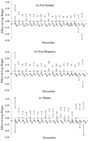
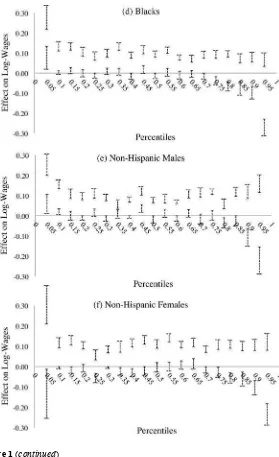
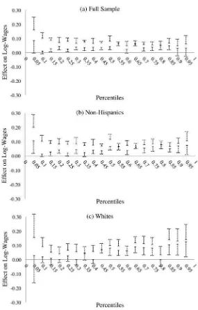
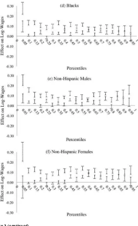
Our empirical results characterize the heterogeneous impact of JC training at differ-ent points of the wage distribution. The estimated bounds for a sample that excludes the group of Hispanics suggest positive effects of JC on wages, both at the mean and throughout the wage distribution. For the various non- Hispanic demographic groups analyzed, the statistically signifi cant estimated average effects are bounded between 4.6 and 12 percent, while the statistically signifi cant quantile treatment effects are bounded between 2.7 and 14 percent. Our analysis by race and gender reveals that the positive effects for blacks appear larger in the lower half of their wage distribution, while for whites the effects appear larger in the upper half of their wage distribution. Non- Hispanic females in the lower part of their wage distribution do not show statisti-cally signifi cant positive effects of JC on their wages, while those in the upper part do. Lastly, our set of estimated bounds for Hispanics are wide and include zero.3
The paper is organized as follows. Section II presents the sample selection problem and the Horowitz and Manski (2000) bounds. Sections III and IV discuss, respectively, bounds on average and quantile treatment effects, as well as the additional assump-tions we consider. Section V describes the JC program and the NJCS, and Section VI presents the empirical results from our application. Section VII concludes.
II. Sample Selection and the Horowitz- Manski Bounds
We describe the sample selection problem in the context of estimating the causal effect of a training program (for example, JC) on wages, where the problem arises because —even in the presence of random assignment—only the wages of those employed are observed. Formally, consider having access to data on N individuals and defi ne a binary treatment Ti, which indicates whether individual i has participated in the program (Ti = 1) or not (Ti = 0). We start with the following assumption:
Assumption A. Ti is randomly assigned.
To illustrate the sample selection problem, assume for the moment that the indi-vidual’s wage is a linear function of a constant term, the treatment indicator Ti and a set of pretreatment characteristics X1i.4
(1) Y*i =β0+Tiβ1+ X1iβ2+U1i,
where Y*i is the latent wage for individual i, which is observed conditional on the self- selection process into employment. This process is also assumed (for the moment) to be linearly related to a constant, the treatment indicator Ti and a set of pretreatment characteristics X2i,
(2) S*i =δ0+Tiδ1+ X2iδ2 +U2i,
Similarly, S*iis a latent variable representing the individual’s propensity to be em-ployed. Let Si denote the observed employment indicator that takes values Si= 1 if individual i is employed and 0 otherwise. Then, Si =1[S*i ≥ 0]=1, where 1[·] is an indicator function. Therefore, we observe individual i’s wage, Yi, when i is employed (Si = 1) and it remains latent when unemployed (Si = 0). In this setting, which assumes treatment effects are constant over the population, the parameter of interest is β1.
Conventionally, point identifi cation of β1 requires strong assumptions such as joint independence of the errors (U1i,U2i) in the wage and employment equations and the regressors T1, X1i, and X2i, plus bivariate normality of (U1i,U2i) (Heckman 1979). The bivariate normality assumption about the errors can be relaxed by relying on exclusion restrictions (Heckman 1990; Imbens and Angrist 1994), which requires variables that determine employment but do not affect wages, or equivalently, variables in X2ithat do not belong in X1i. However, it is well known that fi nding such variables that go along with economic reasoning in this situation is extremely diffi cult (Angrist and Krueger 1999, 2001). More generally, in many economic applications it is diffi cult to fi nd valid exclusion restrictions.
An alternative approach suggests that the parameters can be bounded without rely-ing on distributional assumptions or on the availability and validity of exclusion re-strictions. Horowitz and Manski (2000; HM hereafter) proposed a general framework to construct bounds on treatment effects when data are missing due to a nonrandom process, such as self- selection into nonemployment (S*i < 0), provided that the out-come variable has a bounded support.
To illustrate HM’s bounds, let Yi(0) and Yi(1) be the potential (counterfactual) wages for unit i under control (Ti = 0) and treatment (Ti= 1), respectively. The relationship between these potential wages and the observed Yi is that Yi = Yi(1)Ti+Yi(0)(1−Ti). Defi ne the average treatment effect (ATE) as:
(3) ATE= E[Yi(1)−Yi(0)]= E[Yi(1)]− E[Yi(0)].
Conditional on Ti and the observed employment indicator Si, the ATE in Equation 3 can be written as:
(4) ATE= E[Yi |Ti =1,Si =1] Pr(Si= 1 |Ti =1)
+E[Yi(1) |Ti =1,Si = 0] Pr(Si = 0 |Ti= 1) −E[Yi|Ti = 0,Si =1] Pr(Si= 1 |Ti = 0) −E[Yi(0) |Ti = 0,Si = 0] Pr(Si= 0 |Ti = 0).
.
Examination of Equation 4 reveals that, under random assignment, we can identify from the data all the conditional probabilities (Pr(Si = s|Ti = t), for (t, s) = (0, 1)) and also the expectations of the wage when conditioning on Si=1 (E[Yi|Ti =1,Si =1] and
E[Yi|Ti= 0,Si =1]). Sample selection into nonemployment makes it impossible to point identify E[Yi(1) |Ti =1,Si = 0] and E[Yi(0) |Ti= 0,Si= 0]. We can, however, construct HM bounds on these unobserved objects provided that the support of the outcome lies in a bounded interval [YLB,YUB], because this implies that the values for
these unobserved objects are restricted to such interval. Thus, HM’s upper and lower bounds ( UBHMand
(5) UBHM
= E[Yi|Ti =1,Si =1] Pr(Si =1 |Ti= 1)+YUBPr(S
i = 0 |Ti =1) −E[Yi|Ti = 0,Si= 1] Pr(Si =1 |Ti = 0)−YLBPr(S
i= 0 |Ti = 0) LBHM
= E[Yi|Ti= 1,Si =1] Pr(Si =1 |Ti =1)+YLBPr(S
i = 0 |Ti =1) −E[Yi|Ti = 0,Si= 1] Pr(Si =1 |Ti = 0)−YUBPr(S
i = 0 |Ti = 0).
Note that these bounds do not employ distributional or exclusion restrictions as-sumptions. They are nonparametric and allow for heterogeneous treatment effects— that is, nonconstant effects over the population. On the other hand, a cost of imposing only Assumption A and boundedness of the outcome is that the HM bounds are often wide. Indeed, this is the case in our application, as will be shown below. For this rea-son, we take this approach as a building block and proceed by imposing more structure through the use of assumptions that are typically weaker than the distributional and exclusion restriction assumptions needed for point identifi cation.
III. Bounds on Average Treatment Effects
Lee (2009) and Zhang, Rubin, and Mealli (2008) employ monotonic-ity assumptions that lead to a trimming procedure that tightens the HM bounds. They implicitly or explicitly employ the principal stratifi cation framework of Frangakis and Rubin (2002) to motivate and derive their results. Principal stratifi cation provides a framework for analyzing causal effects when controlling for a posttreatment variable that has been affected by treatment assignment. In the context of analyzing the effect of JC on wages, the affected posttreatment variable is employment. In this frame-work, individuals are classifi ed into “principal strata” based on the potential values of employment under each treatment arm. Comparisons of outcomes by treatment assignment within strata can be interpreted as causal effects because which strata an individual belongs to is not affected by treatment assignment.
More formally, let the potential values of employment be denoted by Si(0) and Si(1)
when i is assigned to control and treatment, respectively. We can partition the popula-tion into strata based on the values of the vector {Si(0),Si(1)}. Because both Si and Ti are binary, there are four principal strata defi ned as NN : {Si(0) = 0,Si(1) = 0}, EE :
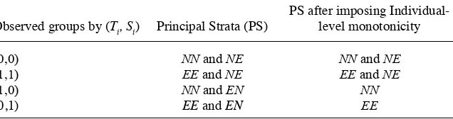
{Si(0) =1,Si(1) =1}, EN : {Si(0) =1,Si(1) = 0}, and NE : {Si(0) = 0,Si(1) =1}. In the context of the application to JC, NN is the stratum of those individuals who would not be employed regardless of treatment assignment, while EE is the stratum of those who would be employed regardless of treatment assignment. The stratum EN represents those who would be employed if assigned to control but unemployed if assigned to treatment, and NE is the stratum of those who would be unemployed if assigned to control but employed if assigned to treatment. Given that strata are defi ned based on the potential values of Si, the stratum an individual belongs to is unobserved. A map-ping of the observed groups based on (Ti,Si) to the unobserved strata above is depicted in the fi rst two columns of Table 1.
observed under both treatment arms, and thus fewer assumptions are required to con-struct bounds for its effects. The average treatment effect for this stratum, which we also consider, is:
(6) ATEEE = E[Yi(1) |EE]− E[Yi(0) |EE].
A. Bounds Adding Individual- Level Monotonicity
To tighten the HM bounds, we employ the following individual- level monotonicity assumption about the relationship between the treatment (JC) and the selection indica-tor (employment):
Assumption B. Individual- Level Positive Weak Monotonicity of S in T: Si(1) ≥ Si(0) for all i.
This assumption states that treatment assignment can affect selection in only one di-rection, effectively ruling out the EN stratum. Both Lee (2009) and Zhang, Rubin, and Mealli (2008) employed this assumption, and similar assumptions are widely used in the instrumental variable (Imbens and Angrist 1994) and partial identifi cation litera-tures (Manski and Pepper 2000; Bhattacharya, Shaikh, and Vytlacil 2008; Flores and Flores- Lagunes 2010). Although Assumption B is directly untestable, Assumptions A and B imply (but are not implied by) E[Si|Ti =1]− E[Si|Ti = 0]≥0, which provides a testable implication for Assumption B (Imai 2008) in settings where Assumption A holds by design, as in our application. In other words, if the testable implication is not satisfi ed, then Assumption B is not consistent with the data. If it is satisfi ed, it only means that the data is consistent with this particular testable implication, However, it does not imply that Assumption B is valid. Thus, this testable implication is not to be interpreted as a statistical test of Assumption B.
[image:7.432.50.368.113.197.2]In the context of JC, Assumption B seems plausible because one of the program’s stated goals is to increase the employability of participants. It does so by providing academic, vocational, and social skills training to participants, as well as job- search assistance. Indeed, the NJCS reported a positive and highly statistically signifi cant av-erage effect of JC on employment of four percentage points (Schochet, Burghardt, and Glazerman 2001). Nevertheless, because this assumption is imposed at the individual
Table 1
Observed Groups Based on Treatment and Employment Indicators (Ti, Si) and Principal Strata (PS) Mixture Within Groups.
Observed groups by (Ti, Si) Principal Strata (PS)
PS after imposing Individual- level monotonicity
(0,0) NN and NE NN and NE
(1,1) EE and NE EE and NE
(1,0) NN and EN NN
level, it may be hard to satisfy as it requires that no individual has a negative effect of the program on employment (or, more generally, on selection).
Two factors that may cast doubt on this assumption in our application are that indi-viduals are “locked- in” away from employment while undergoing training (van Ours 2004), and the possibility that trained individuals may have a higher reservation wage after training and thus may choose to remain unemployed (see, for example, Blundell et al. 2007). Note, however, that these two factors become less relevant the longer the time horizon after randomization at which the outcome is measured. For this reason, in Section VI we focus on wages at the 208th week after random assignment, which is the latest wage measure available in the NJCS.5 In addition, there is one demographic group in our sample for which Assumption B is more likely to be violated. Hispan-ics in the NJCS were the only group found to have negative but statistically insig-nifi cant mean effects of JC on earnings and employment of –$15.1 and –3.1 percent, respectively (Schochet, Burghardt, and Glazerman 2001; Flores- Lagunes, Gonzalez, and Neumann 2010). Although this does not show that the testable implication of Assumption B is statistically rejected for Hispanics, it casts doubt on the validity of this assumption for this group. Thus, we conduct a separate analysis for Hispanics that does not employ Assumption B in Section VIG.
Assumption B, by virtue of eliminating the EN stratum, allows the identifi cation of some individuals in the EE and NN strata, as can be seen after deleting the EN stratum in the last column of Table 1. Furthermore, the combination of Assumptions A and B point identifi es the proportions of each principal stratum in the population. Let πk be the population proportions of each principal stratum, k = NN, EE, EN, NE, and let
ps|t ≡ Pr(Si= s|Ti = t) for t, s = 0,1. Then, πEE = p1|0, πNN = p0|1, πNE = p1|1− p1|0 = p0|0− p0|1, and πEN = 0. Looking at the last column of Table 1, we know that indi-viduals in the observed group with (Ti, Si) = (0,1) belong to the stratum of interest EE. Therefore, we can point identify E[Yi(0) |EE] in Equation 6 as E[Yi|Ti= 0,Si =1]. However, it is not possible to point identify E[Yi(1) |EE], because the observed group with (Ti, Si) = (1,1) is a mixture of individuals from two strata, EE and NE. Neverthe-less, it can be bounded. Write E[Yi|Ti= 1,Si =1] as a weighted average of individuals belonging to the EE and NE strata:
(7) E[Yi|Ti= 1,Si =1]= πEE
(πEE+ πNE)E[Yi(1) |EE]+ πNE
(πEE +πNE)E[Yi(1) |NE].
Because the proportion of EE individuals in the group (Ti,Si) = (1,1) can be point- identifi ed as πEE / (πEE+ πNE) = p1|0/ p1|1, E[Yi(1) |EE] can be bounded from
above by the expected value of Yi for the (p1|0 / p1|1) fraction of the largest values of Yi
in the observed group (Ti,Si) = (1, 1). In other words, the upper bound is obtained under the scenario that the largest (p1|0 / p1|1) values of Yi belong to the EE individuals. Thus, computing the expected value of Yi after trimming the lower tail of the distribu-tion of Yi in (Ti, Si) = (1, 1) by 1 − (p1|0 / p1|1) yields an upper bound for the EE group. Similarly, E[Yi(1) |EE] can be bounded from below by the expected value of Yi for the (p1|0/ p1|1) fraction of the smallest values of Yi for those in the same observed group.
The resulting upper (UBEE) and lower (LBEE) bounds for ATEEE are (Lee 2009; Zhang, Rubin, and Mealli 2008):
(8) UBEE = E[Yi |Ti =1,Si= 1,Yi≥ y1−(p
1|0 /p1|1)
11 ]− E[Y
i |Ti = 0,Si =1]
LBEE = E[Yi|Ti =1,Si =1,Yi ≤ y(p
1|0 /p1|1)
11 ]− E[Y
i|Ti = 0,Si =1],
where y1−(p
1 | 0/p1 |1)
11 and y
(p1 | 0/p1 |1)
11 denote the 1 − (p
1|0/ p1|1) and the (p1|0 / p1|1) quantiles of
Yi conditional on Ti = 1 and Si = 1, respectively. Lee (2009) shows that these bounds are sharp (that is, there are no shorter bounds possible under the current assump-tions).
The bounds in Equation 8 can be estimated with sample analogs:
(9) UBpEE = Yi⋅Ti⋅Si⋅1[Yi ≥ y1−pˆ
p] i=1
n
∑
Ti⋅Si⋅1[Yi ≥ py1−ˆp] i=1
n
∑
−Yi⋅(1−Ti)⋅Si i=1
n
∑
(1−Ti)⋅Si i=1
n
∑
LBEE
p = i=1Yi⋅Ti⋅Si⋅1[Yi ≤ nypˆ]
n
∑
Ti⋅Si⋅1[Yi ≤ ynˆp] i=1
n
∑
−Yi⋅(1−Ti)⋅Si i=1
n
∑
(1−Ti)⋅Si i=1
n
∑
,where yp1−pˆ and nypˆ are the sample analogs of the quantities y1−(p1|0/p1|1)
11 and y
(p1|0/p1|1) 11 in (8),
respectively, and pˆ, the sample analog of (p1|0 / p1|1), is calculated as follows:
(10) pˆ = i=1(1−Ti)⋅Si
n
∑
(1−Ti) i=1
n
∑
/Ti⋅Si i=1
n
∑
Ti i=1
n
∑
.Lee (2009) shows that these estimators are asymptotically normal.
B. Tightening the Bounds by Adding Weak Monotonicity of Mean Potential Outcomes Across Strata
We present a weak monotonicity assumption of mean potential outcomes across the EE and NE strata that tightens the bounds in Equation 8. This assumption was origi-nally proposed by Zhang and Rubin (2003) and employed in Zhang, Rubin, and Mealli (2008):
Assumption C. Weak Monotonicity of Mean Potential Outcomes Across the EE and NE Strata:
E[Y(1) |EE] ≥ E[Y(1) |NE].
the average of pretreatment covariates that are highly correlated with wages between the EE and NE strata, as we illustrate in Section VIB below.
Employing Assumptions A, B, and C results in tighter bounds. To see this, recall that the average outcome in the observed group with (Ti, Si) = (1, 1) contains units from two strata, EE and NE, and can be written as the weighted average shown in Equation 7. By replacing E[Y(1) | NE] with E[Y(1) |EE] in Equation 7 and using the inequality in Assumption C, we have that E[Yi|Ti =1,Si =1]≤ E[Yi(1) | EE], and thus that E[Y(1) |EE] is bounded from below by E[Yi|Ti =1,Si =1]. Therefore, the lower bound for ATEEE becomes: E[Yi|Ti =1,Si =1]−E[Yi|Ti = 0,Si= 1]. Imai (2008) shows that these bounds are sharp.
To estimate the bounds under Assumptions A, B, and C, note that the upper bound estimator of Equation 8 remains UBpEE from Equation 9, although the estima-tor of the lower bound is the corresponding sample analog of E[Yi|Ti= 1,Si =1]− E[Yi|Ti= 0,Si =1]:
(11) LBpEEC
= i=1Yi⋅Ti⋅Si
n
∑
Ti⋅Si i=1
n
∑
−Yi⋅(1−Ti)⋅Si i=1
n
∑
(1−Ti)⋅Si i=1
n
∑
.C. Narrowing Bounds on ATEEE Using a Covariate
Under Assumptions A and B, Lee (2009) shows that (i) grouping the sample based on the values of a pretreatment covariate X, (ii) applying the trimming procedure to con-struct bounds for each group, and (iii) averaging the bounds across these groups, re-sults in narrower bounds for ATEEEas compared to those in Equation 8. This result follows from the properties of trimmed means, and thus it is applicable only to bounds that involve trimming.6
Let X take values on {x1, ....,xJ}. By the law of iterated expectations, we can write the nonpoint identifi ed term in Equation 6 as:
(12) E[Yi(1) |EE]= EX{E[Yi(1) | EE, Xi= xj] |EE}.
Recall from Equation 8 that the bounds on E[Yi(1) |EE] without employing X are given by E[Yi|Ti= 1,Si =1,Yi≥ y1−(p
1|0/p1|1)
11 ]≥ E[Y
i(1) |EE] ≥ E[Yi|Ti =1,Si =1,Y ,Yi ≤ y(p
1|0/p1|1)
11 ]. Thus, it is straightforward to construct bounds on the terms
E[Yi(1) |EE, Xi = xj] for the different values of X by implementing the trimming bounds on E[Yi(1) |EE] discussed in Sections IIIA within cells with Xi = xj. Let these bounds be denoted by LBEEY(1)(x
j) and UBEE Y(1)(x
j), so that UBEE Y(1)(x
j) ≥ E[Yi(1) |EE, Xi= xj] ≥ LBEEY(1)(x
j). It is important to note that the trimming proportions will differ
across groups with different values of X, as the conditional probabilities ps|t are now computed within cells with Xi= xj. After substituting the trimming bounds on
E[Yi(1) |EE, Xi = xj] into Equation 12 we obtain the bounds on ATEEE, which are given by
(13) UB*EE = EX{UBEEY(1)(x
j) |EE}− E[Yi|Ti= 0,Si =1] LB*EE = EX{LBEEY(1)(x
j) | EE}− E[Yi|Ti = 0,Si =1]
Lee (2009) shows that, under Assumptions A and B, these bounds are sharp and that, as compared to those in Equation 8, UB*EE ≤UBEE and LB*EE ≥ LBEE.
An important step in the computation of the bounds in Equation 13 is the estimation of the term Pr(X = xj|EE) used in computing the outer expectation in the fi rst term. By Bayes’ rule, we can write Pr(X = xj|EE) = πEE(xj)⋅Pr(X = xj) / [∑jj=1π
EE(xj)⋅Pr(X = xj)], where πEE(xj) = Pr(EE | X = xj) is the EE stratum
pro-portion in the cell X = xj. Thus, the sample analog estimators of the bounds in Equa-tion 13 are:
(14) UBpEE*
= UBoEE Y(1)
(xj)Prn(X = xj|EE)− j=1
J
∑
i=1Yi⋅(1−Ti)⋅Si n∑
(1−Ti)⋅Si i=1
n
∑
LBEE*
p
= LBoEE Y(1)
(xj)Prn(X = xj|EE)− j=1
J
∑
Yi⋅(1−Ti)⋅Sii=1
n
∑
(1−Ti)⋅Si i=1
n
∑
,where UBoEE Y(1)
(xj) and LBoEE Y(1)
(xj) are the estimators of UBEEY(1)(x
j) and LBEE Y(1)(x
j),
respec-tively, which are computed using the estimators of the bounds on E[Yi(1) |EE] in the fi rst term of Equation 9 for individuals with Xi = xj , and
(15) Prn(X = xj|EE)
= [ i=1(1−Ti)⋅Si⋅
n
∑
1[Xi= xj] / ( (1−Ti)⋅i=1
n
∑
1[Xi= xj])][ 1[Xi =xj]i=1
n
∑
]{[ (1−Ti)⋅Si⋅ i=1
n
∑
1[Xi=xj] / ( (1−Ti)⋅i=1
n
∑
1[Xi =xj])][ 1[Xi= xj]i=1
n
∑
]}j=1
J
∑
.Finally, under Assumptions A, B and C the procedure above is only applied to the upper bound on ATEEE, as the lower bound does not involve trimming.
IV. Bounds on Quantile Treatment Effects
We now extend the results presented in the previous section to con-struct bounds on quantile treatment effects (QTE) based on results by Imai (2008). The parameters of interest are differences in the quantiles of the marginal distributions of the potential outcomes Y(1) and Y(0); more specifi cally, we defi ne the α- quantile effect for the EE stratum:
(16) QTEEEα = FYi−(1)|1EE(α)− F
Yi−(0)|EE
1 (α),
where FYi−(1t)|EE(α) denotes the α- quantile of the distribution of Y
i(t) for the EE stratum.
the distribution of wages of individuals observed employed and unemployed, whereby the wages of employed individuals are assumed to weakly dominate those of unem-ployed individuals (that is, positive selection into employment). In addition, they ex-plore the use of exclusion restrictions to further tighten their bounds. Lechner and Melly (2010) analyze QTE of a German training program on wages. They impose an individual- level monotonicity assumption similar to our Assumption B, and employ the stochastic dominance assumption of Blundell et al. (2007) to tighten their bounds. In contrast to those papers, we take advantage of the randomization in the NJCS to estimate QTE by employing individual- level monotonicity (Assumption B) and by strengthening Assumption C to stochastic dominance applied to the EE and NE strata. Another difference is the parameters of interest: Blundell et al. (2007) focus on the population QTE, Lechner and Melly (2010) focus on the QTE for those individuals who are employed under treatment, and our focus is on the QTE for individuals who are employed regardless of treatment assignment.7
Let FY
i|Ti=t,Si=s(⋅) be the cumulative distribution of individuals’ wages conditional on Ti = t and Si = s, and let yαts denote its corresponding α- quantile, for α∈ (0,1), or
yαts = FY
i|Ti=t,Si=s
−1 (α). Under Assumptions A and B, we can partially identify QTE
EEα as LBEEα ≤ QTEEEα ≤UBEEα , where (Imai 2008):
(17) UBEEα = FY
i|Ti=1,Si=1,Yi≥y1−(p1|0 /p1|1)
1 1
−1 (α)− F
Yi|Ti=0,Si=1
−1 (α)
LBEEα = F
Yi|Ti=1,Si=1,Yi≤y(p1|0 /p1|1) 1 1
−1 (α)− F
Yi|Ti=0,Si=1
−1 (α).
The intuition behind this result is the same as that for the bounds on ATEEE in Equa-tion 8.
F
Yi|Ti=1,Si=1,Yi≥y
1−(p1|0 /p1|1)
11
−1 (α)
and
F
Yi|Ti=1,Si=1,Yi≤y
(p1|0 /p1|1)
11
−1 (α)
correspond to the α- quantile of Yi after trimming, respectively, the lower and upper tail of the distribution of Yi in (Ti,Si) = (1, 1) by 1 − (p1|0 / p1|1), and thus they provide an upper and lower bound for FY
i(1)|EE
−1 (α) in Equation 16. Similar to Equation 8, the quan-tile FY
i(0)|EE
−1 (α) is point identifi ed from the group with (T
i, Si) = (0, 1). Imai (2008)
shows that the bounds in Equation 17 are sharp.
Using the same notation as in Equation 9, we estimate the bounds in Equation 17 using their sample analogs:
(18) UBpEEα = min y:
Ti⋅Si⋅1[Yi≥ y
1−pn p]⋅1[Y
i≤ y] i=1
n
∑
Ti⋅Si⋅1[Yi ≥ y
1−pn p] i=1
n
∑
≥ α ⎧ ⎨ ⎪ ⎩⎪ ⎫ ⎬ ⎪ ⎭⎪−min y: i=1(1−Ti)⋅Si⋅1[Yi ≤ y]
n
∑
(1−Ti)⋅Si i=1
n
∑
≥ α ⎧ ⎨ ⎪ ⎩⎪ ⎫ ⎬ ⎪ ⎭⎪LBEEα
p = min y: Ti⋅Si⋅1[Yi ≤ ypn n]⋅1[Y
i≤ y] i=1
n
∑
Ti⋅Si⋅1[Yi ≤ y p
n
n] i=1
n
∑
≥ α ⎧ ⎨ ⎪ ⎩⎪ ⎫ ⎬ ⎪ ⎭⎪−min y: i=1(1−Ti)⋅Si⋅1[Yi ≤ y]
n
∑
(1−Ti)⋅Si i=1
n
∑
≥ α ⎧ ⎨ ⎪ ⎩⎪ ⎫ ⎬ ⎪ ⎭⎪ .A. Tightening Bounds on QTEEEα Using Stochastic Dominance
We tighten the bounds in Equation 17 by strengthening Assumption C to stochastic dominance. Let FY
i(1)|EE
(⋅) and FY i(1)|NE
(⋅) denote the cumulative distributions of Yi(1) for individuals who belong to the EE and NE strata, respectively:
Assumption D. Stochastic Dominance Between the EE and NE Strata: FY
i(1)|EE(y) ≤ FYi(1)|NE(y), for all y.
This assumption directly imposes restrictions on the distribution of potential outcomes under treatment for individuals in the EE stratum, which results in a tighter lower bound relative to that in Equation 17. Under Assumptions A, B, and D, the resulting sharp bounds are (Imai 2008): LBEEdα ≤ QTE
EEα ≤UBEEα , where UBEEα is as in Equation 17 and
(19) LBEEdα = FY
i|Ti=1,Si=1
−1 (α)− F
Yi|Ti=0,Si=1
−1 (α).
The estimator of the upper bound is still given UBpEEα by in Equation 18, while the estimator for LBEEdα is now given by:
(20) LBpEEdα
= min y: i=1Ti⋅Si⋅1[Yi ≤ y]
n
∑
Ti⋅Si i=1
n
∑
≥ α ⎧ ⎨ ⎪ ⎩⎪ ⎫ ⎬ ⎪ ⎭⎪−min y: i=1(1−Ti)⋅Si⋅1[Yi ≤ y]
n
∑
(1−Ti)⋅Si i=1
n
∑
≥ α ⎧ ⎨ ⎪ ⎩⎪ ⎫ ⎬ ⎪ ⎭⎪B. Narrowing Bounds on QTEEEα Using a Covariate
In this section we propose a way to use a pretreatment covariate X taking values on
{x1, ....,xJ} to narrow the trimming bounds on FY i(1)|EE
−1 (α) and, thus, the bounds on QTE
EEα
in Equation 17. The idea is similar to that in Lee (2009) described in Section III.C, however, the nonlinear form of the quantile function FY
i(1)|EE
diffi culty, we fi rst focus on the cumulative distribution function (CDF) of Yi(1) for the stratum EE at a given point y, FY
i(1)|EE(y) , and write it as the mean of an indicator
func-tion, which allows us to use iterated expectations. A similar approach was also used in Lechner and Melly (2010) to control for selection into treatment based on covariates. Using this insight we can write:
(21) FY
i(1)|EE(y) = E[1[Yi(1)≤ y] | EE]= EX{E[1[Yi(1) ≤ y] | EE, Xi = xj] | EE}. Note that Equation 21 is similar to Equation 12, except that we now employ
1[Yi(1) ≤ y] as the outcome instead of Yi(1). Thus, the methods discussed in Section IIIC (and more generally, the trimming bounds in Section IIIA) can be used to bound
FY
i(1)|EE(y) . As in Section IIIC, let UBEE
y (x
j) and LBEE
y (x
j) denote the upper and lower
bounds on E[1[Yi(1) ≤ y] | EE, Xi = xj] under Assumptions A and B, which are just the trimming bounds on E[Yi(1) |EE] in the fi rst part of Equation 8 within cells with
Xi= xj and employing as outcome the indicator 1[Yi(1) ≤ y] instead of Yi. After substi-tuting UBEEy (x
j) and LBEE
y (x
j) into (21) we obtain the following upper and lower bounds
on FY
i(1)|EE(y) under Assumptions A and B: (22) FUB(y) = EX{UBEEy (x
j) |EE}
FLB(y) = EX{LBEEy (x j) |EE}.
Importantly, by the results in Lee (2009) discussed in Section IIIC, these trimming bounds on FY
i(1)|EE(y) are sharp and tighter than those not employing the covariate X. Given bounds on FY
i(1)|EE(y) for all y ∈ ℜ, the lower (upper) bound on the α- quantile of Yi(1) for the EE stratum, FY
i(1)|EE
−1 (α), is obtained by inverting the upper (lower) bound on FY
i(1)|EE(y) . Using the bounds on FYi(1)|EE(y) in (22), the lower and upper bounds on FY
i(1)|EE
−1 (α) are obtained by
fi nding the value yα such that FUB(yα) = α and FLB(yα) = α,
respectively.8 Therefore, the bounds on QTE
EE
α under Assumptions A and B are given by:
(23) UBEE*α
= FLB−1(α)− F
Yi|Ti=0,Si=1
−1 (α)
LBEE*α
= FUB−1(α)− F
Yi|Ti=0,Si=1
−1 (α).
We implement this procedure by estimating the bounds on FY
i(1)|EE(y) in (22) at M different values of y spanning the support of the outcome, and then inverting the re-sulting estimated bounds to obtain the estimate of the bounds on the α- quantile
FY i(1)|EE
−1 (α). This last set of estimated bounds are then combined with the estimate of
FY i|Ti=0,Si=1
−1 (α) to compute estimates of the bounds on QTE
EE
α in (23). The bounds on
FY
i(1)|EE(ym) at each point ym (m = 1, . . . , M) in (22) are estimated employing the esti-mators of the bounds on E[Yi(1) |EE] in the fi rst term of (9) for individuals with
Xi= xj and using as outcome the indicator function 1[Yi(1)≤ ym] instead of Yi. Finally, just as in the case of the ATEEE in Section III.C, under Assumptions A, B and D, the procedure above is only applied to the upper bound because the lower bound does not involve trimming.
V. Job Corps and the National Job Corps Study
We employ the methods described in the previous sections to assess the effect of Job Corps (JC) on the wages of participants. JC is America’s largest and most comprehensive education and job training program. It is federally funded and currently administered by the U.S. Department of Labor. With a yearly cost of about $1.5 billion, JC annual enrollment ascends to 100,000 students (U.S. Department of Labor 2010). The program’s goal is to help disadvantaged young people, ages 16 to 24, improve the quality of their lives by enhancing their labor market opportunities and educational skills set. Eligible participants receive academic, vocational, and so-cial skills training at over 123 centers nationwide (U.S. Department of Labor 2010), where they typically reside. Participants are selected based on several criteria, includ-ing age, legal U.S. residency, economically disadvantage status, livinclud-ing in a disruptive environment, in need of additional education or training, and be judged to have the capability and aspirations to participate in JC (Schochet, Burghardt, and Glazerman 2001).
Being the nation’s largest job training program, the effectiveness of JC has been debated at times. During the mid- 1990s, the U.S. Department of Labor funded the National Job Corps Study (NJCS) to determine the program’s effectiveness. The main feature of the study was its random assignment: Individuals were taken from nearly all JC’s outreach and admissions agencies located in the 48 continuous states and the Dis-trict of Columbia and randomly assigned to treatment and control groups. From a ran-domly selected research sample of 15,386 fi rst time eligible applicants, approximately 61 percent were assigned to the treatment group (9,409) and 39 percent to the control group (5,977), during the sample intake period from November 1994 to February 1996. After recording their data through a baseline interview for both treatment and control experimental groups, a series of followup interviews were conducted at weeks 52, 130, and 208 after randomization (Schochet, Burghardt, and Glazerman 2001).
Randomization took place before participants’ assignment to a JC center. As a result, only 73 percent of the individuals randomly assigned to the treatment group actually enrolled in JC. Also, about 1.4 percent of the individuals assigned to the control group enrolled in the program despite the three- year embargo imposed on them (Schochet, Burghardt, and Glazerman 2001). Therefore, in the presence of this noncompliance, the comparison of outcomes by random assignment to the treatment has the interpretation of the “intention- to- treat” (ITT) effect—that is, the causal ef-fect of being offered participation in JC. Focusing on this parameter in the presence of noncompliance is common practice in the literature (see, for example, Lee 2009; Flores- Lagunes, Gonzalez, and Neumann 2010; Zhang, Rubin, and Mealli 2009). Cor-respondingly, our empirical analysis estimates nonparametric bounds for ITT effects, although for simplicity we describe our results in the context of treatment effects.
Our sample is restricted to individuals who have nonmissing values for weekly earnings and weekly hours worked for every week after random assignment, resulting in a sample size of 9,145.9 This is the same sample employed by Lee (2009), which facilitates comparing the informational content of our additional assumption
tion C) to tighten the estimated bounds. We also analyze the wage effects of JC for the following demographic groups: non- Hispanics, blacks, whites, non- Hispanic males, non- Hispanic females, and Hispanics. As we further discuss in Section VIA, we sepa-rate Hispanics in order to increase the likelihood that Assumption B holds. Finally, we employ the NJCS design weights (Schochet 2001) throughout the analysis, because different subgroups in the population had different probabilities of being included in the research sample.
A potential concern with the NJCS data is measurement error (ME) in the variables of interest (wages, employment, and random assignment) and the extent to which it may affect our estimated bounds. Although random assignment (T) is likely to be measured without error, both employment (S) and wages (Y) are self- reported and thus more likely to suffer from this problem. In principle, it is hard to know a priori the effect of ME on the estimated bounds, although accounting for plausible forms of ME will likely lead to wider bounds.10 Note that ME in S may lead to misclassifi cation of individuals into strata, affecting the trimming proportions of the bounds involving trimming, while ME in Y will likely affect the trimmed distributions and their mo-ments.
Summary statistics of selected variables for the full sample of 9,145 individuals, by treatment assignment, are presented in Table 2.11 This sample can be characterized as follows: Females comprise around 45 percent of the sample; blacks account for 50 percent of the sample, followed by whites with 27 percent, and by the ethnic group of Hispanics with 17 percent. As expected, given the randomization, the distribution of pretreatment characteristics in the sample is similar between treatment and control groups, with almost all of the differences in the means of both groups being not sta-tistically signifi cant at a 5 percent level (last two columns of Table 2). Importantly, the mean difference is not statistically signifi cant for earnings in the year prior to randomization, which is the covariate (X) employed in Sections VIC and VIF to nar-row bounds. The corresponding differences in labor market outcomes at Week 208 after randomization for this sample is consistent with the previously found positive effect of JC on participants’ weekly earnings of 12 percent and the positive effect on employment of four percentage points (Schochet, Burghardt, and Glazerman 2001).
The unadjusted difference in log wages 208 weeks after random assignment (our outcome of interest Y) equals 0.037 and is statistically signifi cant. This naïve esti-mate of the average effect of JC on wages is affected by sample selection bias, since the treatment, JC training, simultaneously affects both the outcome (log wages) and whether or not the outcome is observed (employment). In what follows, we present estimated bounds on the effect of JC on participants’ wages that account for selection into employment.
10. We are unaware of work assessing the effect of ME on estimated bounds that do not account for this feature of the data. A growing literature that employs bounding techniques to deal with ME includes Horowitz and Manski (1995), Bollinger (1996), Molinari (2008), and Gundersen, Kreider, and Pepper (2012). Extend-ing the bounds in this paper to account for ME is beyond its scope.
Blanco, Flores, and Flores-Lagunes
675
Treatment status Difference
Variable Control (Ti = 0) Treatment (Ti = 1) Difference Standard Error
Selected variables at baseline
Female 0.458 0.452 –0.006 0.010
Age 18.800 18.891 0.091** 0.045
White 0.263 0.266 0.002 0.009
Black 0.491 0.493 0.003 0.010
Hispanic 0.172 0.169 –0.003 0.008
Other race 0.074 0.072 –0.002 0.005
Never married 0.916 0.917 0.002 0.006
Married 0.023 0.020 –0.003 0.003
Living together 0.040 0.039 –0.002 0.004
Separated 0.021 0.024 0.003 0.003
Has a child 0.192 0.189 –0.003 0.008
Number of child 0.272 0.274 0.002 0.013
Education 10.105 10.114 0.008 0.032
Selected labor market variables at baseline
Earnings (X) 2814.362 2904.113 89.751 111.140
Have a job 0.192 0.197 0.006 0.008
Months employed 6.032 6.014 –0.018 0.064
Usual hours / week 34.904 35.436 0.532** 0.250
Usual weekly earnings 107.057 114.771 7.714 5.406
Selected variables after random assignment
Employment at Week 208 (S) 0.566 0.607 0.041*** 0.010
Log wages at Week 208 (Y) 1.991 2.028 0.037*** 0.011
Observations 3,599 5,546
[image:17.432.65.612.56.366.2]VI. Bounds on the Effect of Job Corps on Wages
We start by presenting the HM bounds, which are the basis for the other bounds discussed in Sections III and IV. To construct bounds on the average treatment effect of JC on wages, the HM bounds combine the random assignment in the NJCS (Assumption A) with the empirical bounds of the outcome (log wages at Week 208 after randomization). The empirical upper bound on the support of log wages at Week 208, denoted by YUB in Equation 5, is 5.99; while the lower bound,
YLB,
is –1.55. Using the expressions in Equation 5, the HM bounds are UBHM= 3.135 and
LBHM= −3.109, with a width of 6.244. Clearly, these bounds are wide and largely
un-informative. In what follows, we add assumptions to tighten them.
A. Bounds on ATEEE Adding Individual- Level Monotonicity
Under individual- level monotonicity of JC on employment (Assumption B) we par-tially identify the average effect of JC on wages for those individuals who are em-ployed regardless of treatment assignment (the EE stratum). Therefore, it is of interest to estimate the size of that stratum relative to the full population, which can be done under Assumptions A and B. Table 3 reports the estimated strata proportions for the full sample and for the demographic groups we consider. The EE stratum accounts for close to 57 percent of the population, making it the largest stratum. The second largest stratum is the “never employed” or NN, accounting for 39 percent of the population. Lastly, the NE stratum accounts for 4 percent (the stratum EN is ruled out by Assump-tion B). The relative magnitudes of the strata largely hold for all demographic groups (except NE for Hispanics). Interestingly, whites have the highest proportion of EE individuals at 66 percent, while blacks have the lowest at 51 percent.
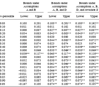
The fi rst column in Panel A of Table 4 reports estimated bounds for ATEEE for the full sample using Equation 9 under Assumptions A and B.12 Relative to the HM bounds, these bounds are much tighter: their width goes from 6.244 in the HM bounds to 0.121. Unlike the HM bounds, the present bounding procedure does not depend on the em-pirical support of the outcome. However, the bounds still include zero, as do the Imbens and Manski (2004; IM hereafter) confi dence intervals reported in the last row of the panel. These confi dence intervals include the true parameter of interest with a 95 per-cent probability. Thus, although Assumption B greatly tightens the HM bounds, it is not enough to rule out zero or a small negative effect of JC on log wages at Week 208.
As discussed in Section IIIA, the untestable individual- level weak monotonicity assumption of the effect of JC on employment may be dubious in certain circum-stances. In the context of JC, it has been documented that Hispanics in the NJCS exhibited negative (albeit not statistically signifi cant) average effects of JC on both their employment and weekly earnings, although for the other groups these effects were positive and highly statistically signifi cant (Schochet, Burghardt, and Glazerman 2001; Flores- Lagunes, Gonzalez, and Neumann 2010). Although this evidence does not show that the testable implication of Assumption B discussed in Section IIIA is statistically rejected for Hispanics, it casts doubt on the validity of Assumption B for
Blanco, Flores, and Flores-Lagunes
677
PS Full Sample Non- Hispanics Whites Blacks Non- Hispanic Males Non- Hispanic Females Hispanics
EE 0.566 0.559 0.657 0.512 0.583 0.530 0.598
NN 0.393 0.392 0.303 0.436 0.377 0.410 0.400
NE 0.041 0.049 0.040 0.052 0.040 0.060 0.002
Observations 9,145 7,573 2,358 4,566 4,280 3,293 1,572
[image:19.432.62.582.177.253.2]The Journal of Human Resources
Table 4
Bounds on the Average Treatment Effect of the EE Stratum for Log Wages at Week 208, by Demographic Groups
Full Sample Non- Hispanics Whites Blacks
Non- Hispanic Females
Non- Hispanic Males
Panel A—Under Assumptions A and B
Upper bound 0.099 0.118 0.120 0.116 0.120 0.114
(0.014) (0.015) (0.028) (0.020) (0.024) (0.020)
Lower bound –0.022 –0.018 0.000 –0.012 –0.023 –0.009
(0.016) (0.017) (0.031) (0.021) (0.026) (0.023)
Width 0.121 0.136 0.120 0.129 0.143 0.123
95 percent IM confi dence interval
[–0.049, 0.122] [–0.046, 0.143] [–0.050, 0.166] [–0.047, 0.149] [–0.066, 0.159] [–0.047, 0.147]
Panel B—Under Assumptions A, B, and C
Upper bound 0.099 0.118 0.120 0.116 0.120 0.114
(0.014) (0.015) (0.028) (0.020) (0.024) (0.020)
Lower bound 0.037 0.050 0.056 0.053 0.046 0.052
(0.012) (0.013) (0.022) (0.016) (0.020) (0.016)
Width 0.062 0.068 0.064 0.063 0.074 0.061
95 percent IM confi dence interval
[0.018, 0.122] [0.029, 0.143] [0.019, 0.166] [0.027, 0.149] [0.014, 0.159] [0.026, 0.147]
this group. Therefore, we consider a sample that excludes Hispanics, as well as other Non- Hispanic demographic groups (whites, blacks, non- Hispanic males, and non- Hispanic females). We defer the analysis of Hispanics that does not employ Assump-tion B to SecAssump-tion VIG, where we also discuss other features of this group in the NJCS. The remaining columns in Panel A of Table 4 present estimated bounds under As-sumptions A and B for various demographic groups, along with their width and 95 percent IM confi dence intervals. The second column presents the corresponding esti-mated bounds for the non- Hispanics sample. The upper bound for this group is larger than the one for the full sample, while the lower bound is less negative, which is consistent with the discussion above regarding Hispanics. The IM confi dence intervals are wider for the non- Hispanics sample relative to the full sample, but they are more concentrated on the positive side of the real line. For the other groups (whites, blacks, and non- Hispanic females and males), none of the estimated bounds exclude zero, although whites and non- Hispanic males have a lower bound almost right at zero. In general, the IM confi dence intervals for the last four demographic groups are wider than those of the full sample and non- Hispanics groups, which is a consequence of their smaller sample sizes.
We now check the testable implication of Assumption B mentioned in Section IIIA:
E(Si|Ti =1)− E(Si|Ti = 0) ≥ 0. The left- hand- side of this expression is the propor-tion of individuals in the NE stratum (πNE), which is reported in Table 3 for all groups. From that table, it can be seen that for all non- Hispanic groups the estimated NE stratum proportions are between 0.04 and 0.06, and they are statistically signifi cant at a 1 percent level (not shown in the table). For Hispanics, however, the corresponding proportion is a statistically insignifi cant 0.002. Thus, while the testable implication of Assumption B is strongly satisfi ed for all non- Hispanic groups, the data does not pro-vide epro-vidence in favor of it for Hispanics, making Assumption B dubious for this de-mographic group.
We close this section by noting, as does Lee (2009), that small and negative esti-mated lower bounds on the effect of JC on wages under the current assumptions can be interpreted as pointing toward positive effects. The reason is that the lower bound is obtained by placing individuals in the EE stratum at the bottom of the outcome dis-tribution of the observed group with (Ti, Si) = (1, 1). Although this mathematically identifi es a valid lower bound, it implies a perfect negative correlation between em-ployment and wages that is implausible from the standpoint of standard models of labor supply, in which individuals with higher predicted wages are more likely to be employed. Indeed, one interpretation that can be given to Assumption C (employed in the next section) is that of formalizing this theoretical notion to tighten the lower bound.
B. Bounds on ATEEE Adding Weak Monotonicity of Mean Potential Outcomes Across Strata
negative effects of JC training on log wages at Week 208. Looking at the IM confi -dence intervals on the bounds adding Assumption C, we see that with 95 percent confi dence the estimated effect is positive. Thus, the effect of JC on log wages at Week 208 for EE individuals is statistically positive and between 3.7 and 9.9 percent. Note that the naïve estimate from Table 2 is numerically equivalent to the lower bound un-der Assumptions A, B and C, which indicates that failing to account for sample selec-tion likely yields an underestimate of the true effect, under the current assumpselec-tions.
Comparing the fi rst and second columns in Panel B of Table 4, it can be seen that the full sample and non- Hispanics have estimated bounds of similar width, although the bounds for non- Hispanics are shifted higher to an effect of JC on wages between 5 to 11.8 percent. The IM confi dence intervals show that, despite the smaller sample size of non- Hispanics, this average effect is statistically signifi cant with 95 percent confi dence. The estimated bounds for the other demographic groups show some in-teresting results. All of the bounds and IM confi dence intervals exclude zero, with the smallest lower bound being that of the full sample at 3.7 percent (all others are 4.6 percent and higher). Remarkably, the estimated bounds for all the demographic groups that exclude Hispanics are relatively similar, suggesting that their average effect of JC on wages for the EE stratum is between 4.6 and 12 percent. The differences in the confi dence intervals across groups are likely driven by the differences in sample sizes. Overall, these results suggest positive average effects of JC on wages across the non- Hispanic demographic groups, and they reinforce the notion of a strong identifying power of Assumption C.
Given the strong identifying power of Assumption C, it is important to gauge its plausibility. Although a direct statistical test is not feasible, we can indirectly gauge its plausibility by looking at one of its implications. Assumption C formalizes the idea that the EE stratum possesses traits that result in better labor market outcomes relative to individuals in the NE stratum. Thus, we look at pretreatment covariates that are highly correlated with log wages at Week 208 and test whether, on average, individuals in the EE stratum indeed exhibit better characteristics at baseline relative to individuals in the NE stratum. We focus mainly on the following pretreatment vari-ables: earnings, whether the individual held a job, months employed (all three in the year prior to randomization), and education at randomization.
To implement this idea, we compute average pretreatment characteristics (W) for the EE and NE strata. Computing average characteristics for the EE stratum is straightforward because, under Assumptions A and B, the individuals in the ob-served group (Ti, Si) = (0, 1) belong to and are representative of this stratum. Simi-larly, the mean E[W |NN] can be estimated from the individuals with (Ti, Si) = (1, 0), who belong to and are representative of the NN stratum. To estimate average characteristics for the NE stratum, note that their average can be written as a func-tion of the averages of the whole populafunc-tion and the other strata, all of which can be estimat