Economic Status of Married Couples
Stephen Wu
a b s t r a c t
This paper uses measures of exogenous health ‘‘shocks’’ to identify the different channels through which changes in health conditions affect in-come, wealth, and consumption behavior. The results indicate that serious health conditions have strong effects on household wealth, but that the ef-fects for women are larger and more significant than the efef-fects for men. The source of the asymmetry arises from the fact that general living ex-penses increase when wives become seriously ill, while for husbands, health shocks do not affect these expenditures.
I. Introduction
Much has been made in the literature about the relationship between health and socioeconomic status (SES), but there is still a great deal to be learned about how the two are linked. Causality from one factor to the other is often difficult to show and the fact that the two may be jointly determined by other ‘‘third factors’’ compounds the problem. While there is strong evidence that there are pathways leading both from SES to health and from health to SES (Smith and Kington 1997; Smith 1999), distinguishing among the factors that influence health and economic outcomes is not an easy task.
A large amount of research has been dedicated to analyzing the health-wealth gradient. There are studies that analyze the relationship between income inequality and health outcomes (Wilkinson 1996; Deaton and Paxson 1999), socioeconomic status and infant mortality (Meara 1998), and behavioral patterns such as smoking and income levels (Marmot, Shipley, and Rose 1984). McClellan (1998) finds that
Stephen Wu is an assistant professor of economics at Hamilton College. The author would like to thank Anne Case, Angus Deaton, Jeffrey Kling, Helen Levy, Harvey Rosen, seminar participants at Hamilton College and Princeton University, and two anonymous referees for helpful comments and sug-gestions. The data used in this article can be obtained August 2003 through July 2006 from Stephen Wu, Department of Economics, Hamilton College, Clinton, NY 13323.
[Submitted July 2000, accepted June 2001]
ISSN 022-166 X2003 by the Board of Regents of the University of Wisconsin System
wealth is related to whether or not there is a new occurrence of a health condition, but his results establish only a cross-sectional correlation and do not show a causal link from health to wealth. Smith (1998; 1999) also finds that serious health events lead to large declines in household net worth but does not distinguish between the effects of health events for men and women, something that will be shown to be important in the current analysis. This paper uses a sample of married couples de-rived from the first two waves of the Health and Retirement Study (HRS) to look at the effects of health shocks on household wealth, income, and consumption. In particular, I test to see whether the effects for husbands and wives are symmetric by including health shocks to each spouse as separate explanatory variables.1There
are several findings in this study. Health shocks do indeed lead to significant declines in household wealth through the channel of lower earnings for both men and women. However, after controlling for earnings decreases due to changes in labor supply, health shocks to husbands do not have additional effects on household wealth accu-mulation, while health shocks to wives have residual effects not entirely explained by lowered household income. The primary reason for this asymmetry is that new health conditions to wives significantly increase the probability that the couple will draw down assets to pay for general living expenses, while new conditions to hus-bands are not associated with the same decline in assets.
II. Data and Empirical Strategy
In this analysis, I use the first two waves of the recent HRS. This survey is a nationally representative panel of approximately 7,000 households with a primary respondent between the ages of 51 and 61 during the first year of the survey. The survey collects detailed information on health status, retirement deci-sions, wealth, work history, family composition, and health insurance. One important aspect of the data is that for married households, information is collected for both spouses. Most of the research related to the issues of health and retirement has fo-cused on men because earlier data sources do not contain information for both hus-bands and wives.2
The sample includes only married couples that were present at both waves of the study and that remained together at the second wave. This excludes couples that were married at the time of the first wave but divorced or separated between waves. It also excludes households where one of the spouses died in the interim period. While the effect of widowhood on economic status is undoubtedly an important policy question, the current analysis does not focus on this issue.3 The resulting
sample includes slightly less than 4,000 married couples.
I use health ‘‘shocks’’ reported between the two waves of the survey as the
exoge-1. It is important to note that I am focusing on married couples. An analysis of single females and single males may have different theoretical predictions and empirical results than in the case of two potential income earners.
nous measure of health change.4 While self-reported health status and changes in
self-reported health status are often used in studies of this nature, they can only demonstrate correlation, and not causality. An individual may feel that his or her health has improved relative to two years ago, but this may be due to the fact that the household is financially better off than before.5In determining the relevant health
conditions, I define severe health conditions to include heart conditions, strokes, cancers and malignant tumors, lung diseases, and diabetes. Since mild conditions such as high blood pressure and arthritis are not shown to significantly affect eco-nomic status in this study, only the severe conditions mentioned above are used in the empirical analysis.6The primary measure of economic status is total household
wealth, which includes all housing and nonhousing equity.
III. Empirical Results
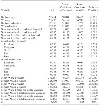
A. Descriptive StatisticsTable 1 shows some summary statistics of the relevant variables. There are 3,826 households in the sample. On average, husbands are approximately four years older than wives and they are slightly more likely to have a new serious health event than wives. Slightly less than 13 percent of all husbands experience a severe condition between periods, while 8.5 percent of wives undergo a new severe condition. The probability of having a new mild health condition (high blood pressure and arthritis) is similar for both men and women (between 11-12 percent). Initial health status is categorized on a self-reported 1-5 scale, with the majority of individuals reporting their health in the first period as excellent, very good, or good. Roughly 6 percent of men and 4 percent of women report being in ‘‘poor’’ health.
B. Health Shocks and Wealth Accumulation
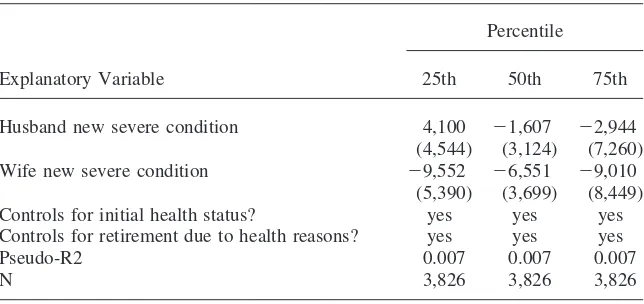
To identify the effects of different channels through which health may affect total wealth, I regress the change in a couple’s assets between Wave 1 and Wave 2 on two indicator variables for the presence of new health shocks – one for health shocks to the husband and one for the wife. Controls for age, race, education, initial health status, and ‘‘forced’’ retirement due to poor health are also included in the regression. Because some of the wealth data are imputed, there are many outliers in the upper tail of the distribution and the use of Ordinary Least Squares yields very imprecise coefficients. To address this issue, I estimate the model using quantile regressions with the change in assets between periods as the dependent variable. The results, shown in Table 2, are quite striking. The effect of a new severe condition to the
4. Other recent papers studying the relationship between health and economic status that use health shocks as an exogenous measure of health change include Charles (1999); Levy (2000); Smith (1999). 5. This is not to say that self-reported measures of health are poor indicators of ‘‘true’’ health status. In fact, most researchers find strong evidence that self-reported health status is highly correlated with morbidity and mortality (see, for example, Idler and Benjamin 1997).
Table 1
Means
Severe Severe
Condition Condition No Severe
Variable All to Husband to Wife Condition
Husband age 57.464 58.841 58.465 57.150
Wife age 53.495 54.167 54.911 53.228
Husband education 12.318 11.889 11.258 12.467
Wife education 12.275 11.872 11.357 12.407
New severe health condition: husband 0.127 1.000 0.169 0.000
New severe health condition: wife 0.085 0.113 1.000 0.000
New mild health condition: husband 0.113 0.151 0.126 0.106
New mild health condition: wife 0.124 0.122 0.154 0.122
Initial health: husband
Excellent 0.230 0.099 0.206 0.251
Very good 0.293 0.204 0.209 0.313
Good 0.294 0.303 0.320 0.291
Fair 0.121 0.239 0.154 0.099
Poor 0.062 0.155 0.111 0.045
Initial health: wife
Excellent 0.260 0.204 0.086 0.283
Very good 0.311 0.278 0.234 0.322
Good 0.267 0.301 0.289 0.260
Fair 0.118 0.157 0.237 0.103
Poor 0.044 0.060 0.154 0.032
Mean Wave 1 wealth 272,187 187,204 209,953 289,843
Median Wave 1 wealth 128,000 94,000 94,500 135,800
Mean Wave 2 wealth 276,091 236,108 197,504 288,832
Median Wave 2 wealth 137,752 101,034 85,296 148,631
Mean Wave 1 total household earnings 38,221 30,929 28,619 40,102 Median Wave 1 total household earnings 34,000 25,000 23,000 36,000 Mean Wave 2 total household earnings 34,952 25,598 24,386 37,199 Median Wave 2 total household earnings 27,454 17,041 16,094 30,112
N 3,826 485 325 3,071
Table 2
Quantile Regressions of Health Shocks and Wealth Changes Dependent Variable is (Wave 2 Wealth)-(Wave 1 Wealth)
Percentile
Explanatory Variable 25th 50th 75th
Husband new severe condition 4,100 ⫺1,607 ⫺2,944
(4,544) (3,124) (7,260)
Wife new severe condition ⫺9,552 ⫺6,551 ⫺9,010
(5,390) (3,699) (8,449)
Controls for initial health status? yes yes yes
Controls for retirement due to health reasons? yes yes yes
Pseudo-R2 0.007 0.007 0.007
N 3,826 3,826 3,826
Note: All regressions include controls for age, education and race. Standard errors in parentheses.
wife is estimated to reduce household wealth by $6,500 to $9,500 (depending on the percentile used in the regression). The coefficients for the 25thpercentile and the
50thpercentile are significant at the 10 percent level.7The median regression shows
that a new severe condition to the husband decreases household wealth by only $1,600, and the coefficient is not statistically different from zero. The results are also insignificant for the 25thand 75thpercentiles. There are large declines in
house-hold wealth associated with new health events to the wife, over and above the effects through the channel of retirement. However, after controlling for baseline health status and retirement effects, health shocks to husbands lead to no significant change in household wealth. For husbands, the effects of health changes on assets are com-pletely absorbed by initial health conditions and changes in retirement decisions, while for wives, there are large effects even after controlling for these variables.
In results not reported here, these regressions have been estimated separately for the subsamples of white couples and black couples, and the results are similar. These results are also robust to different specifications that include a full set of dichotomous age variables (as opposed to just linear terms) and other subsets of explanatory vari-ables. An alternative method of measuring the effects of exogenous changes in health status on wealth accumulation is to use the specific medical conditions as instruments for self-reported health status in the second period. Once again, the results are similar to those reported in Table 2. Exogenous changes in a wife’s health status significantly affect household wealth accumulation, while the analogous effects for exogenous changes in a husband’s health status are much smaller and not statistically significant. For the most part, the general findings reported here are not sensitive to the chosen specification.
C. Alternative Ways of Measuring Health Shocks
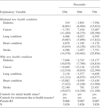
A possible explanation for the differences in the magnitude and significance of these effects is that men and women experience different health conditions. If, for example, it is the case that women have relatively more heart conditions and fewer cases of diabetes, and that for men the reverse is true, it would not be surprising that health shocks to women lead to larger declines in wealth than health shocks to men. In order to deal with the fact that the types of health shocks may differ by sex, I repeat the analysis of Table 2 using specific medical conditions as separate regressors in the equations. The results are reported in Table 3. For wives, heart conditions and cancer are the conditions that lead to the largest drops to total wealth. The median regression shows that heart conditions to a wife lead to a decrease in total wealth of almost $9,000, once again controlling for baseline health status and retirement effects, and the coefficient is significant at the 10 percent level. New onsets of cancer to a wife lead to a decrease of over $13,000 in total wealth, all else constant, though the standard error on this coefficient is fairly large. The results for the 25thand 75th
percentiles are similar. By contrast, the effect on household wealth for every one of the health conditions to husbands is statistically insignificant.
Another possible explanation is that similar medical conditions affect men and women differently. For example, a heart condition may affect a husband’s functional status differently than a wife’s functional status. However, the raw correlation coef-ficients between specific medical conditions and the ability to perform regular daily activities are similar for both men and women. The results (not reported here) indi-cate that all medical conditions have deleterious effects on an index of functional capacity based on the presence of limitations that prevent an individual from doing specific tasks, but the magnitudes of these effects are similar for both husbands and wives.
D. Changes in Earnings and Medical Expenses
Table 3
Quantile Regressions of Specific Health Shocks and Wealth Changes Dependent Variable is (Wave 2 Wealth)-(Wave 1 Wealth)
Percentile
Explanatory Variable 25th 50th 75th
Husband new health condition
Diabetes 319 ⫺3,891 ⫺7,594
(8,801) (6,404) (15,623)
Cancer ⫺1,755 7,410 13,467
(11,450) (8,275) (20,398)
Lung condition 4,486 ⫺8,023 6,595
(9,987) (7,099) (17,832)
Heart condition 4,870 ⫺1,185 ⫺5,178
(5,819) (4,150) (10,172)
Stroke 4,588 ⫺1,057 ⫺7,751
(14,478) (10,462) (25,856)
Wife new health condition
Diabetes ⫺7,048 ⫺2,747 ⫺15,177
(10,878) (7,789) (18,834)
Cancer ⫺14,049 ⫺13,116 ⫺22,470
(12,510) (9,019) (22,399)
Lung condition 2,118 ⫺3,577 ⫺6,658
(11,213) (8,075) (19,577)
Heart condition ⫺15,082 ⫺8,959 ⫺13,430
(7,422) (5,248) (12,588)
Stroke 12,140 781 21,451
(19,037) (14,250) (31,109)
Controls for initial health status? yes yes yes
Controls for retirement due to health reasons? yes yes yes
Pseudo-R2 0.006 0.007 0.007
N 3,826 3,826 3,826
Note: All regressions include controls for age, education and race. Standard errors in parentheses.
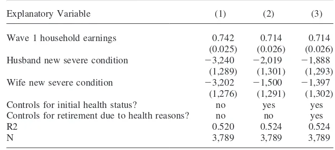
health shock on household income is small, whether the health shock affects the husband or the wife. This finding dispels the notion that the reason that wealth is being drawn down is because people are working less, even if they do not retire. The mean effects of health shocks on yearly household earnings over and above the effects from retirement are approximately $2,000 for both husbands and wives, but neither coefficient is statistically significant.
Table 4
Health Shocks and Earnings Changes
Dependent Variable is Wave 2 Household Earnings
Explanatory Variable (1) (2) (3)
Wave 1 household earnings 0.742 0.714 0.714
(0.025) (0.026) (0.026)
Husband new severe condition ⫺3,240 ⫺2,019 ⫺1,888
(1,289) (1,301) (1,293)
Wife new severe condition ⫺3,202 ⫺1,500 ⫺1,397
(1,276) (1,291) (1,302)
Controls for initial health status? no yes yes
Controls for retirement due to health reasons? no no yes
R2 0.520 0.524 0.524
N 3,789 3,789 3,789
Note: All regressions include controls for age, education and race. Standard errors in parentheses.
the costs incurred by hospital fees, doctor visits, nursing home stays, medical pscriptions, and other related medical expenses. Results (not shown here) from a re-gression of out-of-pocket medical expenditures on health shocks to husbands and wives show that, as expected, medical expenses are well predicted by health shocks. However, there is no asymmetry between the effects for men and women. The mean effects are approximately $2,000 for both husbands and wives. There is still a large decline in wealth due to health shocks to wives that is left unexplained by earnings changes or medical expenses.
E. Household Expenses and the Role of Nonmarket Labor
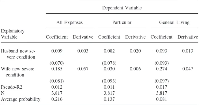
Table 5
Probit Analysis of Health Shocks and the Probability of Drawing from Assets to Pay for Expenses in Wave 2
Dependent Variable
All Expenses Particular General Living
Explanatory
Variable Coefficient Derivative Coefficient Derivative Coefficient Derivative
Husband new se- 0.009 0.003 0.082 0.020 ⫺0.093 ⫺0.013
vere condition
(0.070) (0.078) (0.093)
Wife new severe 0.185 0.057 0.030 0.006 0.274 0.047 condition
(0.081) (0.093) (0.097)
Pseudo-R2 0.012 0.011 0.017
N 3,817 3,817 3,817
Average probability 0.216 0.137 0.081
Note: All regressions include controls for age, education, race, and initial health status. Standard errors in parentheses.
living expenses are considered, a new health event to the wife increases the likelihood of drawing down assets to pay for these expenses by 5 percent (where the average probability is only 8 percent). However, a health shock to the husband still has no effect on the probability of using assets to pay for general expenses. Although the overall probability that households will actually draw into their savings to pay for daily living expenses is not great, this is much more likely to occur if a wife becomes seriously ill.
Rosen-field 1994). Given these facts, it is not surprising that a household is much more likely to draw down assets to pay for general living expenses when a wife becomes ill, but not any more likely when a husband becomes ill. These findings in the sociol-ogy literature are also consistent with the scenario where wives provide home care for their sick husbands, but the reverse is not true.
In analysis not shown here, health shocks to wives lead to significant decreases in liquid wealth. However, health shocks to husbands do not lead to significantly lower levels of liquid wealth. This also supports the hypothesis that health shocks to husbands and wives affect household wealth differently and that the asymmetry is a result of the different effects on household consumption patterns. For wives, health shocks force the household to draw down liquid wealth and assets to pay for expenses, while for husbands, this is not the case. Recently, there have been several studies about the importance of taking into account home production in life-cycle models and studies of labor supply (Baxter and Jermann 1999). When home produc-tion is explicitly modeled, estimates of intertemporal labor supply elasticities are significantly higher than those based on models that ignore home production (Rupert, Rogerson, and Wright 2000). The results here suggest that substitution between work at home and work in the market is much greater for wives whose husbands get sick than for husbands whose wives get sick.
F. Other Considerations
Another possible explanation for the asymmetry of the results is that a health shock to a wife is more of an unexpected event than a health shock to a husband. In this sample of married households, husbands are on average four years older than wives. Given that women also have longer life expectancies than men, it is possible that health events are more of a surprise to a household when the wife becomes ill than when the husband becomes ill. Therefore, households may be more inclined to rap-idly draw down assets in the case where wives experience health shocks. Of course, this is only speculative and an analysis of the expectations of health changes may shed light on this question.
Some cautions to these results are worth noting. The household wealth variables used in this paper do not include any measures of pension wealth. Gustman et al. (1997) show that pension and social security wealth account for significant portions of total household wealth. Perhaps households simply shift wealth from nonhousing and housing equity to pension wealth. However, in some preliminary results not reported here, conditional on the level of total nonhousing and housing assets, health variables are not highly correlated with contributions to pension plans and other retirement plans, or with retirement income received.
IV. Conclusion
The results indicate that health shocks lead to fairly large declines in assets be-tween periods and that these declines are due to a variety of factors. Part of the decrease in household wealth can be attributed to the losses in income due to forced retirement. While this is not surprising, I find that even after controlling for initial health status and labor supply changes, health shocks to wives result in large drops in total wealth (approximately $6,500), while no residual effects are present when husbands become ill. This finding is robust to different empirical specifications and to alternative ways for measuring health changes. Several different types of health events to wives lead to large declines in household wealth, whereas none of the specific conditions to husbands significantly affect total wealth. In addition, medical expenditures cannot fully explain the large decreases in wealth that occur when wives experience health shocks.
One aspect of economic status that is linked to wives’ health events but not to husbands becoming ill is spending on general consumption. There is a much higher probability that a couple will draw from existing assets to pay for general living expenses when a wife becomes ill. However, the likelihood of this happening is unaffected by shocks to a husband’s health. Furthermore, health shocks to wives result in large drops in liquid financial wealth, but no analogous declines are attrib-uted to health events of husbands. Since increases in general consumption would tend to result in smaller amounts in checking and savings accounts, this lends further support to this hypothesis. One possible explanation for the asymmetry of these effects is the fact that nonmarket labor is not accounted for by changes in labor force status. If wives share a large burden of household chores, regardless of labor force status, then it follows that health shocks to wives would lead to declines in household wealth that are not entirely accounted for by changes in earnings.
In terms of policy relevance, these results suggest that health insurance alone may be insufficient for protecting households from the economic effects of serious health conditions. While health insurance may be adequate for paying certain medical ex-penditures, some households may not be well equipped to deal with unexpected health events because of their additional effects on consumption. In particular, health shocks to wives may be very costly to a couple’s financial well being.
References
Baxter, Marianne, and Urban J. Jermann. 1999. ‘‘Household Production and the Excess Sensitivity of Consumption to Current Income.’’American Economic Review 89(4):902-20.
Bielby, Denise D., and William T. Bielby. 1988. ‘‘She Works Hard for the Money: House-hold Responsibilities and the Allocation of Work Effort.’’American Journal of Sociol-ogy93:1031-59.
Bird, Chloe. 1996. ‘‘Gender, Paid and Unpaid Work, and Depression.’’Society for the Study of Social ProblemsAssociation Paper.
Charles, Kerwin K. 1999. ‘‘Sickness in the Family: Health Shocks and Spousal Labor Sup-ply.’’ Ford School of Public Policy Working Paper 00-011, University of Michigan. Deaton, Angus, and Christina Paxson. 1999. ‘‘Mortality, Education, Income, and Inequality
among American Cohorts.’’ NBER Working Paper No. 7140.
1997. ‘‘Pension and Social Security Wealth in the Health Retirement Study.’’ NBER Working Paper No. 5912.
Gustman, Alan L., and Thomas L. Steinmeier. 2000. ‘‘Retirement in Dual Career Families: A Structural Model’’Journal of Labor Economics18(3):503-45.
Hochschild, Arlie, and Anne Machung. 1989.The Second Shift: Working Parents and the Revolution at Home. New York: Academic Press.
Hurd, Michael D. 1990. ‘‘The Joint Retirement Decisions of Husbands and Wives.’’ In Is-sues in the Economics of Aging, ed. David A Wise, 231-54. Chicago: University of Chi-cago Press.
Idler, Ellen L., and Yael Benyamini. 1997. ‘‘Self-Rated Health and Mortality: A Review of Twenty-Seven Community Studies.’’Journal of Health and Social Behavior38(1): 21-37.
Lennon, Mary C., and Sarah Rosenfield. 1994. ‘‘Relative Fairness and the Division of Housework: The Importance of Options.’’American Journal of Sociology 100(2):506-31.
Levy, Helen. 2000. ‘‘The Financial Impact of Health Insurance.’’ UC-Berkeley. Mimeo. Marmot, Michael G., Martin J. Shipley, and Geoffrey Rose. 1984. ‘‘Inequalities in Death:
Specific Explanations of a General Pattern?’’Lancet1(8384):1003-1006.
Meara, Ellen. 1998 ‘‘Why is Health Related to Socioeconomic Status?’’ Harvard Univer-sity Mimeo.
McClellan, Mark. 1998. ‘‘Health Events, Health Insurance, and Labor Supply: Evidence from the Health and Retirement Study.’’In Frontiers in the Economics of Aging, ed. Da-vid A. Wise, 301-52. Chicago: University of Chicago Press.
Rupert, Peter, Richard Rogerson, and Randall Wright. 2000. ‘‘Homework in Labor Eco-nomics: Household Production and Intertemporal Substitution.’’Journal of Monetary Economics46(3):557-79.
Smith, James P. 1998. ‘‘Socioeconomic Status and Health.’’American Economic Review
88(2):192-196.
———. 1999. ‘‘Healthy Bodies and Thick Wallets: The Dual Relation Between Health and Economic Status.’’Journal of Economic Perspectives13(2):145-66.