Distribution Network Optimization Based on Genetic Algorithm
Ramadoni Syahputra
Department of Electrical Engineering, Faculty of Engineering Universitas Muhammadiyah Yogyakarta
Kampus Terpadu UMY, Jl. Lingkar Selatan, Kasihan, Bantul, Yogyakarta 55183 E-mail: [email protected]
Abstract – This paper presents a new robust optimization technique for distribution network configuration, which can be regarded as a modification of the recently developed genetic algorithm. The multi-objective genetic algorithm has been applied to this problem to optimize the total cost while simultaneously minimize the power loss and maximize the voltage profile. The IEEE 69-bus distribution network is used in the tests, and test results have shown that the algorithm can determine the set of optimal non-dominated solutions. It allows the utility to obtain the optimal configuration of the network to achieve the best system with the lowest cost. Copyright © 2017 Universitas
Muhammadiyah Yogyakarta- All rights reserved.
Keywords: Distribution network, Optimization, Network Reconfiguration, Genetic Algorithm, Multi-objective
I.
Introduction
Distribution systems, which are the important component in power system, are normally configured radially for effective coordination of their protective devices [1]-[3]. There are two types of switches in network operation. The switches are generally found in the system for both protection and configuration management [4]-[5]. These are sectionalizing switches (normally closed switches) and tie switches (normally opened switches) [6]-[8]. By changing the status of the sectionalizing and tie switches, the configuration of distribution system is varied and loads are transferred among the feeders while the radial configuration format of electrical supply is still maintained and all load points are not interrupted. This activity is defined as distribution feeder reconfiguration. The advantages obtained from feeder reconfiguration are real power loss reduction, balancing system load, increasing system security and reliability, bus voltage profile improvement, and power quality improvement [9]-[11].
In recent years, power distribution systems have been a significant increase in small-scaled generators, which is known as distributed generator
(DG) [12]-[16]. Distributed generators are grid- connected or stand-alone electric generator units located within the distribution system at or near the end user [17]. Recent development in DG technologies such as wind, solar, fuel cells, hydrogen, and biomass has drawn an attention for utilities to accommodate DG units in their systems [18]-[21]. The introduction of DG units brings a number of technical issues to the system since the distribution network with DG units is no longer passive [22].
The practical aspects of electric power distribution system should also be considered for the implementation of feeder reconfiguration. The actual distribution feeders are primarily unbalanced in nature due to various reasons, i.e., , presence of single, double, and three-phase line sections, unbalanced consumer loadsand existence of asymmetrical line sections [23]-[27]. The inclusion of system unbalances increases the dimension of the feeder configuration problem because all three phases have to be considered instead of a single
phase balanced representation [28]-[30].
Consequently, the analysis of distribution systems necessarily required a power flow algorithm with complete three-phase model [31]-[32].
technique for distribution feeder reconfiguration to improve the performance of the distribution system with the presence of distributed generators. The two objectives to be minimized are real power loss and number of switching operations of tie and sectionalizing switches, while all feeders keep in load balancing. The effectiveness of the methodology is examined by an IEEE distribution system consisting of 69 buses.
II.
Distribution Network Optimization
Distribution network optimization can be done using network reconfiguration. Distribution network reconfiguration is a very important and usable operation to reduce distribution feeder losses and improve system security. The configuration may be varied via switching operations to transfer loads among the feeders. Two types of switches are used: normally closed switches (sectionalizing switches) and normally open switches (tie switches) [8]. By changing the open/close status of the feeder switches load currents can be transferred from feeder to feeder. During a fault, switches are used to fault isolation and service restoration. There are numerous numbers of switches in the distribution system, and the number of possible switching operations is tremendous. Feeder reconfiguration thus becomes a complex decision-making process for dispatchers to follow. There are a number of closed and normally opened switches in a distribution system. The number of possible switching actions makes feeder reconfiguration become a complex decision-making for system operators. Figure 1 shows a schematic diagram of a simplified primary circuit of a distribution system. In the figure, CB1- CB6 are normally closed switches that connect the line sections, and CB7 is a normally open switch that connects two primary feeders. The two substations can be linked by CB8, while CB9, when closed, will create a loop.
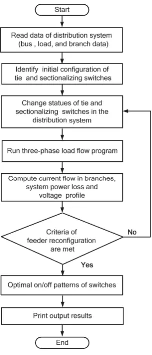
Optimum operation of distribution systems can be achieved by reconfiguring the system to minimize the losses as the operating conditions change. Reconfiguration problem essentially belongs to combinatorial optimization problem because this problem is carried out by taking into account various operational constraints in large scale distribution systems. It is, therefore, difficult to rapidly obtain an exact optimal solution on real system (Chung-Fu, 2008). A flowchart for feeder reconfiguration algorithm is shown in Fig 2.
Fig. 1. Schematic diagram of a distribution system for reconfiguration
Power flow is an essential tool for the steady state operational analysis of power systems. The main objective of power flow analysis is to calculate the real and reactive powers flow in each line as well as the magnitude and phase angle of the voltage at each bus of the system for the specific loading conditions [4]. Certain applications, particularly in distribution automation and
optimization, require repeated power flow
solutions. As the power distribution networks become more and more complex, there is a higher demand for efficient and reliable system operation. Consequently, power flow studies must have the capability to handle various system configurations with adequate accuracy and speed.
Fig. 2. Flowchart of distribution network reconfiguration
The equivalent circuit for each line section could be represented by the nominal -equivalent model. This model has one series and two parallel components. The series component stands for the total line impedance consisting of the line resistance and reactance. The parallel components represent the total line capacitance, which is distributed along the line. In the pi-equivalent line representation, the total line capacitance is equally divided into two parts: one lumped at the receiving end bus and the other at sending end bus while the series line impedance is lumped in between. The series impedance and the shunt capacitance for a three-phase line are 3 × 3 complex matrices which take into account the mutual inductive coupling between the phases.
III.
Genetic Algorithm
A cost function generates an output from a set of input variables (a chromo- some). The cost function
may be a mathematical function, an experiment, or a game. The object is to modify the output in some desirable fashion by finding the appropriate values for the input variables. We do this without thinking when filling a bathtub with water. The cost is the difference between the desired and actual temperatures of the water. The input variables are how much the hot and cold spigots are turned. In this case the cost function is the experimental result from sticking your hand in the water. So we see that deter- mining an appropriate cost function and deciding which variables to use are intimately related. The term fitness is extensively used to designate the output of the objective function in the GA literature. Fitness implies a maximization problem. Although fitness has a closer association with biology than the term cost, we have adopted the term cost, since most of the optimization literature deals with minimization, hence cost. They are equivalent.
The GA begins by defining a chromosome or an array of variable values to be optimized. If the chromosome has Nvar variables (an Nvar-dimensional opti- mization problem) given by p1, p2, . . . , pNvar, then the chromosome is written as an Nvar element row vector.
chromosome = [p1, p2, p3, . . . , pNvar] (1)
For instance, searching for the maximum elevation on a topographical map requires a cost function with input variables of longitude (x) and latitude (y)
chromosome = [x, y] (2)
where Nvar = 2. Each chromosome has a cost found by evaluating the cost func- tion, f, at p1, p2,
… , pNvar:
cost=f (chromosome) = f(p1, p2, …, pNvar) (3) Since we are trying to find the peak in Rocky Mountain National Park, the cost function is written as the negative of the elevation in order to put it into the form of a minimization algorithm:
f (x, y) = -elevation at (x, y) (4)
mileage might include size of the car, size of the engine, and weight of the materials. Other variables, such as paint color and type of headlights, have little or no impact on the car gas mileage and should not be included. Sometimes the correct number and choice of variables comes from experience or trial optimization runs. Other times we have an analytical cost function. A cost function defined by
f (w, x, y, z) = 2x + 3y + z/100000 + 9876
with all variables lying between 1 and 10 can be simplified to help the optimization algorithm. Since the w and z terms are extremely small in the region of interest, they can be discarded for most purposes. Thus the four-dimensional cost function is adequately modeled with two variables in the region of interest.
Most optimization problems require constraints or variable bounds. Allowing the weight of the car to go to zero or letting the car width be 10 meters are impractical variable values. Unconstrained variables can take any value. Constrained variables come in three brands. First, hard limits in the form
of >, <, ≥, and £ can be imposed on the variables. When a variable exceeds a bound, then it is set equal to that bound. If x has limits of 0 £ x £ 10, and the algorithm assigns x = 11, then x will be reassigned to the value of 10. Second, variables can be transformed into new variables that inherently include the constraints. If x has limits of 0 £ x £ 10, then x = 5 sin y + 5 is a transformation between the constrained variable x and the unconstrained variable y. Varying y for any value is the same as varying x within its bounds. This type of trans- formation changes a constrained optimization problem into an unconstrained optimization problem in a smooth manner. Finally there may be a finite set of variable values from which to choose, and all values lie within the region of interest. Such problems come in the form of selecting parts from a limited supply.
Dependent variables present special
problems for optimization algorithms because varying one variable also changes the value of the other variable. For example, size and weight of the car are dependent. Increasing the size of the car will most likely increase the weight as well (unless some other factor, such as type of material, is also changed).
Independent variables, like Fourier series coefficients, do not interact with each other. If 10 coefficients are not enough to represent a function, then more can be added without having to recalculate the original 10.
The GA starts with a group of chromosomes known as the population. The population has
Npop chromosomes and is an Npop ¥ Nbits
matrix filled with random ones and zeros generated using
pop=round(rand(Npop, Nbits));
where the function (Npop, Nbits) generates a
Npop ¥ Nbits matrix of uniform random numbers between zero and one. The function round rounds the numbers to the closest integer which in this case is either 0 or 1. Each row in the pop matrix is a chromosome.
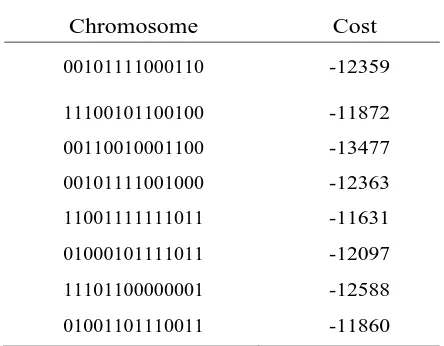
Table 1. Example Initial Population of 8 Random Chromosomes and Their Corresponding Cost
Chromosome Cost
00101111000110 -12359
11100101100100 -11872
00110010001100 -13477
00101111001000 -12363
11001111111011 -11631
01000101111011 -12097
11101100000001 -12588
01001101110011 -11860
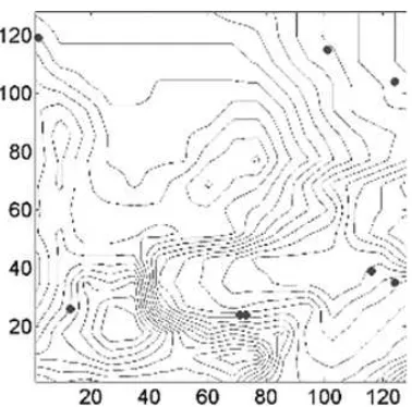
The chromosomes correspond to discrete values of longitude and latitude. Next the variables are passed to the cost function for evaluation. Table 1 shows an example of an initial population and their costs for the Npop
= 8 random chromosomes. The locations of
the chromosomes are shown on the
Fig. 3. A contour map of the cost surface with the 8 initial population members indicated by
large dots
Random mutations alter a certain
percentage of the bits in the list of chromosomes. Mutation is the second way a GA explores a cost surface. It can introduce traits not in the original population and keeps the GA from con- verging too fast before sampling the entire cost surface. A single point mutation changes a 1 to a 0, and vice versa. Mutation points are randomly selected from the Npop ¥ Nbits total number of bits in the population matrix. Increasing the number of
mutations increases the algorithm’s freedom
to search outside the current region of variable space. It also tends to distract the algorithm from converging on a popular solution. Mutations do not occur on the final iteration.
After the mutations take place, the costs associated with the offspring and mutated chromosomes are calculated. The process described is iterated.
The number of generators that evolve depends on whether an acceptable solution is reached or a set number of iterations is exceeded. After a while all the chromosomes and associated costs would become the same if it were not for mutations. At this point the algorithm should be stopped.
Most GAs keeps track of the population statistics in the form of population mean and minimum cost. For our example, after three generations the global minimum is found to be -14199.
IV.
Results and Discussion
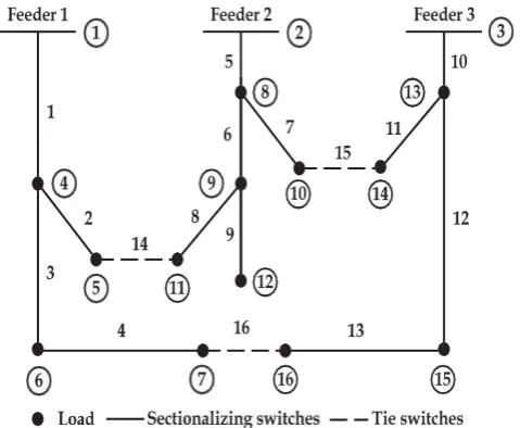
The test system for the case study is a radial distribution system with 69 buses, 7 laterals and 5 tie-lines (looping branches), as shown in Fig. 1. The current carrying capacity of branch No.1-9 is 400 A, No. 46-49 and No. 52-64 are 300 A and the other remaining branches including the tie lines are 200 A.
Fig. 4. The IEEE 69-bus distribution network
sectionalizing switches (switches No. 1-68) are closed while all the tie-switches (switch No. 69-73) open. The total loads for this test system are 3,801.89 kW and 2,694.10 kVAr. The minimum and maximum voltages are set at 0.95 and 1.05 p.u. The maximum iteration for the Tabu search algorithm is 100. The fuzzy parameters associated with the three objectives are given in Table 3.
The numerical results for the six cases are summarized in Table 4. In cases 1-5 (balanced systems), the system power loss and the LBI are highest, and the minimum bus voltage in the system violates the lower limit of 0.95 per unit. The voltage profile of case 1 is shown in Fig. 12. It is observed that the voltages at buses 57-65 are below 0.95 p.u. because a large load of 1,244 kW are drawn at bus 61. Without the four DG units, the system loss would be 673.89 kW. This confirms that DG units can normally, although not necessarily, help reduce current flow in the feeders and hence contributes to power loss reduction, mainly because they are usually placed near the load being supplied. In cases 2 to 5, where the feeders are reconfigured and the voltage constraint is imposed in the optimization process, no bus voltage is found violated (see Figs.12 and 13).
As expected, the system power loss is at minimum in case 2, the LBI index is at minimum in case 3, and the number of switching operations of
switches is at minimum in case 4. It is obviously seen from case 5 that a fuzzy multiobjective optimization offers some flexibility that could be exploited for additional trade-off between improving one objective function and degrading the others. For example, the power loss in case 5 is slightly higher than in case 2 but case 5 needs only 6, instead of 8, switching operations. Although the LBI of case 3 is better than that of case 5, the power loss and number of switching operations of case 3 are greater. Comparing case 4 with case 5, a power loss of about 18 kW can be saved from two more switching operations. It can be concluded that the fuzzy model has a potential for solving the decision making problem in feeder reconfiguration and offers decision makers some flexibility to incorporate their own judgment and priority in the optimization model.
The membership value of case 5 for power loss is 0.961, for load balancing index is 0.697 and for number of switching operations is 0.666.
When the system unbalanced loading is 20% in case 6, the power loss before feeder reconfiguration is about 624.962 kW. The membership value of case 6 for power loss is 0.840, for load balancing index is 0.129 and for the number of switching operations is 0.666.
Table 2. Results of case study
Case 1 Case 2 Case 3 Case 4 Case 5 Case 6
Sectionalizing switches to be open - 12, 20,
52, 61
42, 14,
20, 52, 61 52, 62 13, 52, 63 12, 52 61
Tie switches to be closed - 70, 71, 72, 73 71, 72, 73 69, 70, 72, 73 71, 72, 73 71, 72, 73
Power loss (kW) 586.83 246.33 270.81 302.37 248.40 290.98
Minimum voltage (p.u.) 0.914 0.954 0.954 0.953 0.953 0.965
Load balancing index (LBI) 2.365 1.801 1.748 1.921 1.870 2.273
Number of switching
V.
Conclusion
In this paper, a new approach has been proposed to re- configure and install DG units simultaneously in distribution system. In addition, different loss reduction methods (only network reconfiguration, only DG installation, DG installation after reconfiguration) are also simulated to establish the superiority of the proposed method. An efficient
results show that simultaneous network
reconfiguration and DG installation method is more effective in reducing power loss and improving the voltage profile compared to other methods. The effect of number of DG installation locations on power loss reduction is studied at different load levels. The results show that the percentage power loss reduction is improving as the number of DG installation locations are increasing from one to four, but rate of improvement is decreasing when locations are increased from one to four at all load levels.
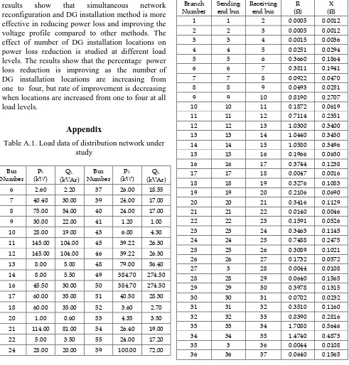
Appendix
Table A.1. Load data of distribution network under study
37 37 38 0.1053 0.1230 Performance Enhancement of Distribution Network with DG Integration Using Modified PSO Algorithm. Journal of Electrical Systems (JES), 12(1), pp. 1-19.
[2] Syahputra, R., Robandi, I., Ashari, M. (2014).
“Optimal Distribution Network Reconfiguration with Penetration of Distributed Energy Resources”,
Proceeding of 2014 1st International Conference on Information Technology, Computer, and Electrical Engineering (ICITACEE) 2014, UNDIP Semarang, pp. 388 - 393.
[3] Syahputra, R., (2012), “Fuzzy Multi-Objective
Approach for the Improvement of Distribution
Network Efficiency by Considering DG”,
International Journal of Computer Science & Information Technology (IJCSIT), Vol. 4, No. 2, pp. 57-68.
[4] Syahputra, R., (2012), “Distributed Generation: State
of the Arts dalam Penyediaan Energi Listrik”, LP3M
UMY, Yogyakarta, 2012.
[5] Syahputra, R., (2016), “Transmisi dan Distribusi
Tenaga Listrik”, LP3M UMY, Yogyakarta, 2016.
[6] Syahputra, R., Robandi, I., Ashari, M. (2014). Optimization of Distribution Network Configuration with Integration of Distributed Energy Resources Using Extended Fuzzy Multi-objective Method. International Review of Electrical Engineering (IREE), 9(3), pp. 629-639.
[7] Syahputra, R. (2016). Application of Neuro-Fuzzy Method for Prediction of Vehicle Fuel Consumption. Journal of Theoretical and Applied Information Technology (JATIT), 86(1), pp. 138-149.
[8] Syahputra, R., Robandi, I., Ashari, M. (2015). Performance Improvement of Radial Distribution Network with Distributed Generation Integration Using Extended Particle Swarm Optimization Algorithm. International Review of Electrical Engineering (IREE), 10(2). pp. 293-304.
[9] Syahputra, R., Robandi, I., Ashari, M. (2015). Reconfiguration of Distribution Network with DER Integration Using PSO Algorithm. TELKOMNIKA, 13(3). pp. 759-766.
[10] Syahputra, R., Robandi, I., Ashari, M. (2015). PSO Based Multi-objective Optimization for Reconfiguration of Radial Distribution Network. International Journal of Applied Engineering Research (IJAER), 10(6), pp. 14573-14586.
[11] Syahputra, R., Robandi, I., Ashari, M., (2012),
“Reconfiguration of Distribution Network with DG
Using Fuzzy Multi-objective Method”, International Conference on Innovation, Management and Technology Research (ICIMTR), May 21-22, 2012, Melacca, Malaysia.
[12] Jamal, A., Syahputra, R. (2012), “Adaptive Neuro -Fuzzy Approach for the Power System Stabilizer Model in Multi-machine Power System”, International Journal of Electrical & Computer Sciences (IJECS), Vol. 12, No. 2, 2012.
[14] Syahputra, R., Robandi, I., Ashari, M. (2014). Performance Analysis of Wind Turbine as a Distributed Generation Unit in Distribution System. International Journal of Computer Science & Information Technology (IJCSIT), Vol. 6, No. 3, pp. 39-56.
[15] Jamal, A., Suripto, S., Syahputra, R. (2015). Multi-Band Power System Stabilizer Model for Power Flow Optimization in Order to Improve Power System Stability. Journal of Theoretical and Applied Information Technology, 80(1), pp. 116-123. [16] Syahputra, R., Soesanti, I. (2016). An Optimal
Tuning of PSS Using AIS Algorithm for Damping Oscillation of Multi-machine Power System. Journal of Theoretical and Applied Information Technology (JATIT), 94(2), pp. 312-326.
[17] Soesanti, I., Syahputra, R. (2016). Batik Production Process Optimization Using Particle Swarm Optimization Method. Journal of Theoretical and Applied Information Technology (JATIT), 86(2), pp. 272-278.
[18] Jamal, A., Syahputra, R. (2016). Heat Exchanger Control Based on Artificial Intelligence Approach. International Journal of Applied Engineering Research (IJAER), 11(16), pp. 9063-9069.
[19] Syahputra, R. (2015). Characteristic Test of Current Transformer Based EMTP Shoftware. Jurnal Teknik Elektro, 1(1), pp. 11-15.
[20] Syahputra, R., Soesanti, I. (2015). Power System Stabilizer model based on Fuzzy-PSO for improving power system stability. 2015 International Conference on Advanced Mechatronics, Intelligent Manufacture, and Industrial Automation (ICAMIMIA), Surabaya, 15-17 Oct. 2015 pp. 121 - 126.
[21] Syahputra, R., Robandi, I., Ashari, M., (2013),
“Distribution Network Efficiency Improvement
Based on Fuzzy Multi-objective Method”. International Seminar on Applied Technology, Science and Arts (APTECS). 2013; pp. 224-229. [22] Syahputra, R., Soesanti, I. (2015). “Control of
Synchronous Generator in Wind Power Systems Using Neuro-Fuzzy Approach”, Proceeding of International Conference on Vocational Education and Electrical Engineering (ICVEE) 2015, UNESA Surabaya, pp. 187-193.
[23] Syahputra, R., (2013), “A Neuro-Fuzzy Approach For the Fault Location Estimation of Unsynchronized Two-Terminal Transmission Lines”, International Journal of Computer Science & Information Technology (IJCSIT), Vol. 5, No. 1, pp. 23-37.
[24] Jamal, A., Syahputra, R. (2013). UPFC Based on Adaptive Neuro-Fuzzy for Power Flow Control of Multimachine Power Systems. International Journal of Engineering Science Invention (IJESI), 2(10), pp. 05-14.
[25] Syahputra, R. (2010). Fault Distance Estimation of Two-Terminal Transmission Lines. Proceedings of International Seminar on Applied Technology, Science, and Arts (2nd APTECS), Surabaya, 21-22 Dec. 2010, pp. 419-423.
[26] Syahputra, R., Soesanti, I. (2016). DFIG Control Scheme of Wind Power Using ANFIS Method in Electrical Power Grid System. International Journal of Applied Engineering Research (IJAER), 11(7), pp. 5256-5262.
[27] Jamal, A., Suripto, S., Syahputra, R. (2016). Performance Evaluation of Wind Turbine with Doubly-Fed Induction Generator. International Journal of Applied Engineering Research (IJAER), 11(7), pp. 4999-5004.
[28] Syahputra, R., Soesanti, I. (2016). Design of Automatic Electric Batik Stove for Batik Industry. Journal of Theoretical and Applied Information Technology (JATIT), 87(1), pp. 167-175.
[29] Jamal, A., Syahputra, R. (2014). Power Flow Control of Power Systems Using UPFC Based on Adaptive Neuro Fuzzy. IPTEK Journal of Proceedings Series. 2014; 1(1): pp. 218-223.
[30] Syahputra, R., Soesanti, I. (2016). Power System Stabilizer Model Using Artificial Immune System for Power System Controlling. International Journal of Applied Engineering Research (IJAER), 11(18), pp. 9269-9278.
[31] Syahputra, R., (2014), “Estimasi Lokasi Gangguan Hubung Singkat pada Saluran Transmisi Tenaga
Listrik”, Jurnal Ilmiah Semesta Teknika Vol. 17, No.
2, pp. 106-115, Nov 2014.
[32] Jamal, A., Syahputra, R., (2011), “Design of Power System Stabilizer Based on Adaptive Neuro-Fuzzy
Method”. International Seminar on Applied
Technology, Science and Arts (APTECS). 2011; pp. 14-21.
Authors’
information
Ramadoni Syahputra received B.Sc. degree