The Minimum Wage, Restaurant
Prices, and Labor Market Structure
Daniel Aaronson
Eric French
James MacDonald
a b s t r a c t
Using store-level and aggregated Consumer Price Index data, we show that restaurant prices rise in response to minimum wage increases under several sources of identifying variation. We introduce a general model of employment determination that implies minimum wage hikes cause prices to rise in competitive labor markets but potentially fall in monopsonistic environments. Furthermore, the model implies employment and prices are always negatively related. Therefore, our empirical results provide evidence against the importance of monopsony power for understanding small observed employment responses to minimum wage changes. Our estimated price responses challenge other explanations of the small employment response, too.
I. Introduction
This paper utilizes unique data to test whether restaurant prices re-spond to minimum wage changes. We find that restaurant prices unambiguously rise
Daniel Aaronson is a senior researcher at the Federal Reserve Bank of Chicago. Eric French is a senior researcher at the Federal Reserve Bank of Chicago. James MacDonald is a senior researcher at the Economic Research Service, U.S. Department of Agriculture. Work on the store-level price data was performed under a memorandum of understanding between the Economic Research Service at the Department of Agriculture and the Bureau of Labor Statistics (BLS), which permitted onsite access to the confidential BLS data used in this paper. The authors thank Bill Cook, Mark Bowman, and Scott Pinkerton of the BLS for their advice and help. They also thank Gadi Barlevy, Jeff Campbell, Bob LaLonde, Derek Neal, Dan Sullivan, and seminar participants at multiple settings for helpful comments and Tina Lam for excellent research assistance. The views expressed herein are not necessarily those of the Federal Reserve Bank of Chicago, Federal Reserve System, Bureau of Labor Statistics, or U.S. Department of Agriculture. Comments welcome at efrench@frbchi.org or daaronson@frbchi.org. The publicly available data (city level aggregates) used in this article can be obtained beginning January 2009 through December 2012 from Daniel Aaronson, Federal Reserve Bank of Chicago, 230 S. LaSalle St., Chicago, IL 60604. Telephone (312)322-5650, Fax (312)322-2357.
[Submitted May 2007; accepted August 2007]
ISSN 022-166X E-ISSN 1548-8004Ó2008 by the Board of Regents of the University of Wisconsin System
after minimum wage increases are enacted.1Furthermore, these price increases are larger for establishments that are more likely to pay the minimum wage. These results are derived from a panel of store-level restaurant prices that are the basis for the food away from home component of the Consumer Price Index (CPI) during a three-year period with two federal minimum wage increases, and are corroborated using a longer panel of city-level food away from home pricing from the CPI.
Because of the breadth of our price data, we can take advantage of several sources of variation. First, some states set their minimum wage above the Federal level. Second, we can distinguish restaurants that tend to pay the minimum wage from those that do not. Third, the fraction of workers paid at or near the minimum wage varies across geo-graphic areas. All three sources of variation indicate that most, if not all, of the higher labor costs faced by employers are pushed onto customers in the form of higher prices. As suggested by Brown (1999), the size and sign of these price responses can be used to infer whether monopsony power is important for understanding the employment re-sponse to minimum wage hikes. The minimum wage literature has become contentious because Card and Krueger’s (for example, 1995, 2000) research found that an increase in the minimum wage has no, or even a small positive, effect on employment. Therefore, their research contradicts standard models of competitive labor markets, which, prior to their work, most researchers suspected was relevant for industries which primarily employed minimum wage workers.2However, their results are consistent with monop-sony power in the labor market, as Stigler (1946) discussed many years ago. The diverse findings reported in the flurry of replies to their work (for example, Neumark and Wascher 1996, 2000; Deere, Murphy, and Welch 1995; Kim and Taylor 1995; Burkhauser, Couch, and Wittenburg 2000; Dickens, Machin, and Manning 1999) led one observer to note that ‘‘½Card and Krueger’slasting contribution may well be to show that we just don’t know how many jobs would be lost if the minimum wage were increased.and that we are unlikely to find out by using more sophisticated methods of inference on the existing body of data. What is needed is more sophisticated data’’ (Kennan 1995).
Restaurant prices complement the existing evidence on employment responses be-cause, as we show below, output prices and employment are unambiguously negatively related in response to an exogenous change in wage rates. In order to show this relation-ship, we introduce a general model of employment determination that allows for a range of output and input market structures. Part of the reasoning behind the negative relationship between output prices and employment is based on the negative relation-ship between prices and output. We also add some weak assumptions to the model to
show that output and labor input are positively related. Therefore, if the output price rises in response to a minimum wage hike, both output and labor input have fallen. This will be the case if labor markets are competitive. Conversely, if the output price falls in response to a minimum wage hike, total output and labor input have increased. This will potentially be the case if firms have monopsony power in the labor market.
Research on monopsony power has recently been revitalized by the empirical and the-oretical work of Card and Krueger (1995), Burdett and Mortenson (1998), Bhaskar and To (1999), Ahn and Arcidiacono (2003), Flinn (2006), Manning (1995), and Rebitzer and Taylor (1995).3But our results suggest that competition is likely more relevant than mo-nopsony. Moreover, in Aaronson and French (2007), we show that a computational model of labor demand with a competitive labor market structure predicts price responses that are comparable to those found in this paper. The employment elasticities that are derived from that calibrated model are within the bounds set by the empirical literature.
To be clear, as Boal and Ransom (1997), among others, point out, our results do not necessarily prove labor markets are competitive. Although the results are clearly consistent with this conclusion, if the minimum wage is set high enough, positive comovement between the minimum wage and prices may be consistent with the mo-nopsony model as well. We discuss this point more formally below.
However, our results provide evidence against the hypothesis that monopsony power is important for understanding the observed small employment responses found in some min-imum wage studies. Indeed, our estimated price responses provide evidence against other explanations of the small employment response as well, including the potential substitution of nonwage for wage compensation and the importance of endogenous work effort or ef-ficiency wages. They do, however, provide support for a model of ‘‘hungry teenagers,’’ whereby higher income resulting from a minimum wage increase causes low-wage workers to buy more minimum wage products, attenuating the disemployment effect of the mini-mum wage. Although our test answers a fairly narrow question, we believe that the answer to this question is of broad interest. Given that the low observed employment responses to minimum wage changes sparked particular interest in the importance of monopsony power in the labor market, our results should temper this interest.
Finally, it is important to emphasize that our estimates are for the restaurant indus-try only. This indusindus-try is a major employer of low-wage labor and therefore a partic-ularly relevant one to study.4However, as a result of different intensities of use of
minimum wage labor, substitution possibilities, market structure, or demand for their products, other industries might face different employment responses. See Aaronson and French (2007) for further details.
II. Data
Under an agreement with the Bureau of Labor Statistics (BLS), we were granted access to the store-level data employed to construct the food away from home component of the CPI during 1995 to 1997.5While the time frame is short, this three-year period contains an unusual amount of minimum wage activity. A bill signed on August 20, 1996 raised the federal minimum from $4.25 to $5.15 per hour, with the increase phased in gradually. An initial increase to $4.75 (11.8 percent) oc-curred on October 1, and the final installment (8.4 percent) took effect on September 1, 1997. Moreover, additional variation can be exploited because price responses will vary geographically. This occurs for two reasons. First, market wages may exceed min-imum wages in some areas but not in others. Second, some states set minmin-imum wages above the federal level. We capture the latter source of heterogeneity by allowing the effective minimum wage to be the maximum of the state and federal level.6
The sample itself is based on nearly 7,500 food items at over 1,000 different estab-lishments in 88 Primary Sampling Units (PSUs).7Because restaurants in some geo-graphic areas are surveyed every other month, all numbers are reported as bimonthly (every other month) price changes.8Within an establishment, specific items, usually seven or eight, are selected for pricing with probability proportional to sales. During our time frame, an ‘‘item’’ usually was a meal, as the BLS aimed to price complete meals as typically purchased (for example, a meal item might consist of a hamburger, french fries, and a soft drink). Our data set codes items broadly, such as breakfast, lunch, dinner, or snacks. Unfortunately, because there are no specific item descrip-tions, we cannot tie price changes to item-specific measures of input price changes (such as ground beef or chicken price indexes). Nevertheless, the BLS strives to price identical items over time, and codes in our database describe temporal item substi-tutions due to discontinuance and alteration. Our analysis focuses on price changes
5. Because the BLS introduced a complete outlet and item resampling in January 1998, we only use data through December 1997. Data prior to 1995 are no longer available. Bils and Klenow (2004) use the same 1995 to 1997 period.
6. This source of variation is especially useful in Section IIIC, when we look at city level variation between 1979 and 1995. During 1995 to 1997, ten states (not including Alaska, which is always $0.50 above the federal level) had minimum wages above the federal level for some part of the period. Six states (HI, MA, NJ, OR, VT, and WA) were at or above the federal minimum of $4.75 prior to October of 1996. Three states (HI, MA, and OR) were at or above the federal minimum prior to September 1997. Further variation is available from states (CA, CT, NJ, WA) that were between the old $4.75 minimum wage but below the new $5.15 minimum wage.
7. The 88 PSUs cover 76 metropolitan statistical areas and 12 other areas representing the urban nonmetro United States.
for identical items, and we do not compare prices where the BLS has made an item substitution.9
A particular advantage of this data is its depiction of the type of business. Limited-service (LS) outlets, which account for roughly 30 percent of the sample, are those stores where meals are served for on- or off-premises consumption and patrons typ-ically place orders and pay at the counter before they eat. Roughly half the sample is comprised of full-service (FS) outlets, establishments that provide wait service, sell food primarily for on-premises consumption, take orders while patrons are seated at a table, booth or counter, and typically ask for payment from patrons after they eat.10 The minimum wage is likely to increase wages at LS restaurants more than at FS restaurants, for two reasons. First, wages for cashiers and crew members are higher, perhaps by 60 percent, at FS restaurants than LS restaurants.11Thus, a higher frac-tion of workers are paid the minimum wage at LS restaurants. Second, many FS employees are paid through tips and the federal tipped minimum wage remained $2.13 throughout our sample period. Thus, minimum wage changes have smaller effects on wages in FS outlets than LS outlets because tip earnings usually exceed effective minimum wages.12
9. Firms could respond to a minimum wage increase by reducing quality, instead of raising price. While we do not have direct measures of quality, the data set notes whether an item is the same as the item priced in the previous month. There is no evidence of any increased incidence of item changes or substitutions fol-lowing minimum wage increases, suggesting that quality changes or item substitution are not a standard means of dealing with a cost shock. There also might be concern that a minimum wage increase changes the composition of items sampled. If revenues are negatively correlated with prices and sampling probabil-ity is a function of sales, a change in the minimum wage could result in a shift in the distribution of sampled products towards high priced items (or stores with fewer minimum wage workers). To minimize this con-cern, we ran everything with sampling weights and found identical results.
10. The BLS replaced an old ordering with these types of business codes in July 1996, and began to report price indexes for type of business groupings after our data period in January 1998. Businesses surveyed early in our sample period were retroactively assigned the new codes. The remaining fifth of non-LS and non-FS outlets, which we usually exclude from this analysis, include meals consumed at department stores, supermarkets, convenience stores, gas stations, vending machines, and many other outlets. 11. Assuming that LS wage rates are identical to U.S. McDonald’s wage rates collected by McKinsey Global Institute and reported in Ashenfelter and Jurajda (2001), then wage rates among cashier and crew members in FS establishments in the outgoing rotation files of the CPS are about 60 percent higher than wage rates in LS establishments. Ashenfelter and Jurajda report the average U.S. McDonald’s wage for crew and cashier workers was $6.00 and $6.50 in December 1998 and August 2000, respectively. We com-pared these figures to the average wage of $7.81 and $8.52 for CPS workers that report their industry as eating and drinking places and their occupation as food preparation and service occupation, janitors and cleaners, or sales counter clerks during the fourth quarter of 1998 or the third quarter of 2000. Assuming all LS establishments pay the same wage as McDonalds and noting that the 1997 Economic Census of Accommodations and Food Services reports that 48 percent of all employees in FS and LS establishments are employed in the LS sector, we can back out that FS establishments pay roughly 60 percent higher hourly wages than LS establishments within these occupation codes. The Economic Census also reports average weekly wages that are approximately 20 percent higher in FS establishments. But this calculation does not correct for differences in hours worked per week and cannot refine the sample by occupational class. 12. Federal law sets a separate cash minimum for tipped employees (which is $2.13 throughout our sample period), but requires that tips plus cash wages must at least equal the nontipped employee minimum. For example, in September 1996, $2.62 ($4.75-$2.13) in tips are allowed to be applied to a tipped employee’s wage to reach the minimum wage. In 1996, only Rhode Island and Vermont changed their state-specific tipped minimum. In 1997, Maryland, Michigan, North Dakota, and Vermont did as well. Of these states, only Maryland and Michigan are included in our CPI sample.
III. Estimates of Price Pass-Through
One problem with price (as well as employment) data is that they are potentially measured with error.13In other words,pijkt¼pijkt+eijkt, wherepijktis the measured price of itemkat outletjin stateiduring montht,pijkt is the model pre-dicted value, where the model is described in Section IV, andeijktis measurement or model misspecification error.14We approach the data in three ways.
A. Store-level Descriptions of Price Increases and Decreases
Our first approach ignores errors in the price data and simply tabulates price increases and decreases after a minimum wage change. In the model described in Section IV, we formally show that price data can be used to infer labor market struc-ture. In particular, price cuts tend to be an outcome unique to monopsonistic labor markets. In the absence of measurement error, observed price cuts allow us to iden-tify individual firms that potentially have monopsony power. On the other hand, if variability in eijkt is significant, measurement or misspecification error may cause us to erroneously infer monopsony power when in fact none exists.
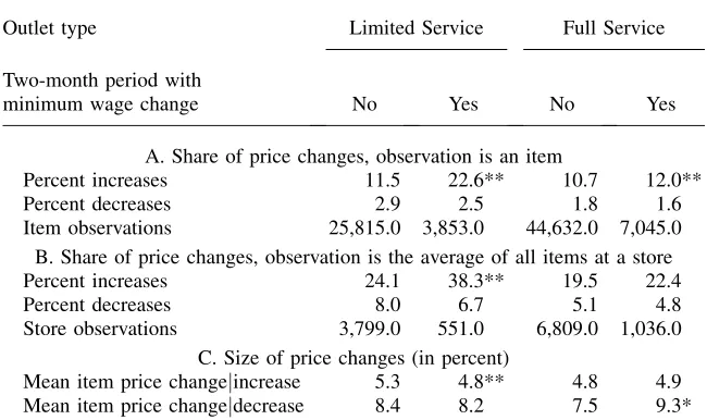
Table 1 reports descriptive statistics on the frequency and size of price changes for Limited-Service (Column 2) and Full-service (Column 4) outlets in the two months immediately after a minimum wage change. For comparison, all other two month periods are reported in Columns 1 and 3. In Panel A, the observational unit is a food item. Because multiple items are surveyed for each store, individual stores are in these computations up to eight times each period. Panel B computes price changes by store. That is, an average price is calculated from each store’s sampled items and consequently a store is included, at most, once every two months.
There are several notable features of the data. First and foremost, prices increase in response to a minimum wage change. During the two months after a minimum wage increase, 22.6 percent of LS items increased in price. This is almost double the 11.5 per-cent share of LS price quotes that are increased in months without a minimum wage increase.15Moreover, as expected, the minimum wage effect is substantially smaller, although still statistically significant, for full-service outlets. In such stores, the share of quotes that are higher than the previous two months is 12 percent, exceeding months that do not follow a minimum wage increase by 1.3 percentage points. Excluding small price changes (say, those less than 2 percent) that might be driven by measurement error reinforces these differences. Price increases over 2 percent are more than twice as likely
13. Measurement error is unlikely to be important in this data (Bils and Klenow 2004). The BLS has procedures in place to flag and investigate unusual observations. Nevertheless, some measurement error may exist for the following three reasons. First, the price on the menu may differ from the price paid because of discounts and cou-pons distributed outside of outlets. Prices are collected net of sales and promotions but some, particularly those not run by the outlet itself may be missed. Second, high frequency but short-term price changes may not be cap-tured by our monthly data (Chevalier, Kashyap, and Rossi 2003). Third, surveyors may falsely report last month’s price instead of going to the restaurant to record the price, a practice known as ‘‘curbstoning.’’ There is no reason to think that any of these sources of error are correlated with the presence of a minimum wage change. 14. There are other interpretations foreijkt, such as menu costs of switching prices. Moreover, many firms
in our sample offer short-term sales for reasons that are unrelated to changes in input prices.
in minimum wage months in LS establishments (17.6 versus 8.6 percent) and 24 per-cent more likely in FS establishments (8.9 versus 7.2 perper-cent).
Conversely, there is little evidence that minimum wage increases cause price declines. The share of prices that decline is stable throughout the three years regardless of whether the minimum wage has been altered. The results are identical when small changes are excluded. Therefore, based on incidence alone, the data suggest that many firms raise their price, but few reduce it, in response to a change in the minimum wage. These results are robust to looking at price movements at the store-level, as reported in Panel B. Here, prices are computed by averaging the price of all items in a store. Again, there is a notable acceleration of LS outlet price increases follow-ing a minimum wage increase (38.3 percent versus 24.1 percent) but no unusual in-crease in price declines during these periods.16
Finally, increasing the frequency of price changes is not the only avenue for firms to raise or lower prices. The size of price changes could be altered as well.17However, Panel C shows that, if anything, price increases tend to be slightly smaller in size after minimum wage increases. The size of LS price cuts are unaffected by minimum wage changes.
Table 1
Means of Selected Variables
Outlet type Limited Service Full Service
Two-month period with
minimum wage change No Yes No Yes
A. Share of price changes, observation is an item
Percent increases 11.5 22.6** 10.7 12.0**
Percent decreases 2.9 2.5 1.8 1.6
Item observations 25,815.0 3,853.0 44,632.0 7,045.0
B. Share of price changes, observation is the average of all items at a store
Percent increases 24.1 38.3** 19.5 22.4
Percent decreases 8.0 6.7 5.1 4.8
Store observations 3,799.0 551.0 6,809.0 1,036.0
C. Size of price changes (in percent)
Mean item price changejincrease 5.3 4.8** 4.8 4.9
Mean item price changejdecrease 8.4 8.2 7.5 9.3*
* (**)¼Statistically different from months without a minimum wage increase at the 5(1) percent level.
16. We have explored looking at longer intervals but are quite limited by our data. The September 1997 in-crease is only four months before the end of our sample, so we are forced to rely on a single comparison: pre- and post- the 1996 increase. The results are a bit more muted but similar inferences can be drawn. LS price hikes in the ten months after October 1996 are 6 percentage points (53 vs. 47 percent) more common than in the average ten month period in the year and a half prior to October 1996. Price declines occur slightly more fre-quently (but not statistically so) in the ten months after the increase: 6 percent versus 5 percent.
There is some evidence of larger price cuts in FS establishments after minimum wage hikes, but this is a rare event (only 1.6 percent of all FS item observations). It is worth noting that, while price cuts (in FS and LS stores) are rare, they can be large. Over a quar-ter of all food away from home price cuts exceed 10 percent, and over a tenth exceed 20 percent. By comparison, price increases are more tightly concentrated, with about half under 4 percent and less than a tenth above 10 percent.18However, there is little evidence that the size of price cuts change in any meaningful way after a minimum wage increase. Kolmogorov-Smirnov D-tests for differences in price distributions finds no significant shift in the size of price cuts following minimum wage increases.19The fact that these large declines exist in roughly the same fashion in nonminimum wage change periods suggests to us that the largest cuts typically reflect temporary sales.
Assuming that all markets are competitive (or, as we point out in Section IVC, fac-tor markets are competitive and product markets are monopolistically competitive) and firms have a constant returns to scale production function, it is straightforward to show that all cost increases will be passed onto consumers in the form of higher prices. If minimum wage labor’s share of total firm costs issmin, then a 10 percent increase in the minimum wage should increase the product pricesmin310 percent. To get a sense of whether the observed price responses are consistent with compe-tition, we note that minimum wage labor’s share of total costs is equal to labor’s share of total costs multiplied by minimum wage labor’s share of labor costs. 10-K company reports, the Economic Census for Accommodations and Foodservices, and the IRS’ Statistics on Income Bulletin all provide an estimate of labor’s share of total costs, and in each, the sample median and mean are around 30 to 35 percent.20Unfortunately,
18. Price changes cluster near the mean, with excess kurtosis of 62.0 and 80.8 for price changes among LS and FS outlets, respectively. Distributions of increases and decreases are also quite peaked compared to normal distributions, with excess kurtosis of 14.2 (LS) and 8.6 (FS) for increases, and 1.6 (LS) and 6.8 (FS) for decreases. Kashyap (1995) also reports positive excess kurtosis in his sample of catalog prices.
we are less certain of minimum wage labor’s share of total labor costs for the average firm. Using household level data, we know that about a third of all restaurant workers are paid near the minimum wage over this time period, constituting 17 percent of all payments to labor.21Using these values, we make two calculations that bound the competitive response. If there is only one type of labor, all firms have the same em-ployment level, and all firms either pay 0 percent of their workers or 100 percent of their workers the minimum wage, depending on the labor market, then 33 percent of all firms pay the minimum wage. Given this, and the fact that about 33 percent of total costs are in the form of labor costs, then a 10 percent increase in the minimum wage raises prices by 10 percent 333 percent333 percent¼1.09 percent. Alternatively, if all firms hire above minimum wage labor in equal proportions, then each restaurant must have 17 percent of its labor costs going to minimum wage labor. Thus, a 10 per-cent increase in the minimum wage should raise prices by 10 perper-cent333 percent3 17 percent¼0.56 percent.
Aaronson and French (2007) use a calibrated model of labor demand that accounts for both firm and worker heterogeneity to show that when these factors are explicitly accounted for, the competitive model predicts prices will increase by roughly 0.7 per-cent. Moreover, because limited-service restaurants are more likely to pay the min-imum wage than full-service restaurants, competition would imply larger price increases at limited-service restaurants. Given that some restaurants do not increase prices after minimum wage hikes, but restaurants that do raise their prices usually do so by more than 0.7 percent, it is difficult to compare the observed price response to the competitive prediction. Section IIIB presents a statistical model to better make this comparison.
B. Estimates of Price Pass-Through
The next approach provides a more complete statistical model of the price response to a minimum wage change. In our basic model we regress the log change in prices for itemkat outletjin periodton the percentage change in the minimum wage in stateiover the contemporaneous, lag, and lead periods, and a set of controls:
Dlnpijkt¼ + H
h¼1
ahDlnpijkt2h+ + 2
h¼0
bhDlnPPIt2h+ + 1
h¼21
vhDlnwmin;it2h+uijkt ð1Þ
We includewmin;it21andwmin;it+ 1to allow a more flexible response to the legisla-tion, as price responses can play out over time. Consider the timing of the 1996–97 federal increase. When the law was passed, firms knew that minimum wages would be increased on October 1, 1996, and again on September 1, 1997. It is conceivable that firms could react to the expectation of an increase (that is, at the bill discussion
21. See Aaronson and French (2007) for a description of this calculation. Because wage distributions are not available in company reports, we estimate the share of employees that are paid at or near the minimum wage from the outgoing rotation files of the CPS for the two years prior to the 1996 legislation. We use a survey in Card and Krueger (1995, p. 162) to account for the share of workers paid slightly above the min-imum wage that are impacted by new legislation.
or passage), rather than the enactment dates. However, empirically, we found no ev-idence of longer leads or lags.22
The vector of controls include contemporaneous and lags of changes in the pro-ducer price index for processed foods to account for material input price shocks faced by sample outlets (lnPPIt).23To allow for mean-reverting price movements that typically occur after sales or price hikes, we also experimented with controls for lags in lnpijkt. However, the minimum wage estimates barely change whether lagged dependent variables are accounted for or not (the version reported in Table 2 includes them).24
Table 2 presents the basic results. Because quotes from the same outlet are un-likely to be statistically independent, all standard errors account for quote (that is, menu items within an establishment) clustering, using Huber-White robust estima-tion techniques. We also checked for error clustering by city, chain, and outlet. While within-outlet effects were important, within-city and within-chain effects were not. All results are reported as elasticities and multiplied by ten to gauge the impact of a 10 percent minimum wage increase.
Column 1 reports the minimum wage effect for the full sample of food away from home establishments. We find that a 10 percent increase in the minimum wage increases prices by roughly 0.7 percent (with a standard error of 0.14), of which over half the response occurs within the first two months after the minimum wage change. However, because this result combines outlets where the minimum wage is binding with those where it might be less important, two particular sources of variation can be used to identify the price response to a minimum wage increase.
First, as in Table 1, we can take advantage of variation in the intensity of minimum wage worker use between limited- (Column 2) and full- (Column 3) service restau-rants. The price increase generated by a 10 percent minimum wage hike is roughly
22. Businesses knew of the 1996 increase just two to four months prior to implementation. They knew of the 1997 increase, specified in the 1996 bill, 13 to 15 months before implementation. The 1996 increase could not have been predicted until shortly before the House of Representatives vote on May 23, after a week of legislative maneuvering that almost consigned the bill to defeat (Weisman 1996 and Rubin 1996). Even then, the final timing of the minimum wage increase did not become clear until adoption of the conference report on August 2. Aaronson (2001) shows that longer-run price pass-through estimates are roughly the same size as short-run estimates using aggregated U.S. and Canadian price data. 23. Aaronson (2001) accounts for the costs of particular food items, such as chicken, beef, bread, cheese, lettuce, tomatoes, and potatoes, and finds similar aggregated results to those reported here. We also con-trolled for broader labor market pressures using changes in CPS median wages and fixed chain and PSU (i.e. city) effects (not shown). Minimum wage point estimates and standard errors are quite robust to the inclusion of these variables. Furthermore, the fixed effects themselves added almost nothing to the model’s fit. Controls for meal type (breakfast, lunch, or dinner) are also included but have no impact on the results. 24. To be clear, the inclusion of a lagged dependent variable potentially leads to inconsistent parameter estimates. In practice, this bias appears to be negligible. But, for completeness, we also ran a specification that included one lag in lnpijktthat is instrumented by thrice-lagged prices and found statistically
Table 2
The Price Response to a 10 Percent Minimum Wage Increase
Variable All
Limited service
Full
service All
Limited service
Limited service
Full service
Full service
Column 1 2 3 4 5 6 7 8
Dlnwmin,it21 0.229 0.334 0.234 0.225 0.295 0.202 0.249 0.246
(0.064) (0.117) (0.082) (0.067) (0.12) (0.326) (0.087) (0.157)
D lnwmin,it 0.407 0.94 0.19 1.444 2.695 2.392 1.039 1.245
(0.07) (0.135) (0.086) (0.531) (0.883) (1.005) (0.692) (0.706)
D lnwmin,it+1 0.077 0.275 20.102 0.078 0.243 0.451 20.082 20.228
(0.063) (0.136) (0.073) (0.067) (0.149) (0.431) (0.079) (0.164)
Dlnwmin,it*wage20 20.161 20.278 20.242 20.128 20.133
(0.078) (0.133) (0.134) (0.1) (0.1) Total effect 0.713 1.549 0.322
(0.14) (0.275) (0.168)
At wage20¼$5.00 0.94 1.84 1.84 0.56 0.6 At wage20¼$7.00 0.62 1.29 1.35 0.31 0.33 At wage20¼$9.00 0.3 0.73 0.87 0.05 0.07
Month dummies? no no no no no yes no yes
Include PPI? yes yes yes yes yes no yes no
R2 0.07 0.167 0.017 0.07 0.171 0.175 0.019 0.021
N 71,077 21,883 36,928 63,630 18,691 18,691 33,875 33,875
Notes: See text for detail. Controls not shown in the table include three lags in lnPijktand meal type (breakfast, lunch, or dinner). Huber-White standard errors corrected
for clustering at the item and establishment level are in parentheses. Sample sizes in Columns 2 and 3 do not add up to Column 1 because some establishments are not categorized as full- or limited-service restaurants. Wage20 is the 20th percentile of the MSA’s hourly wage distribution, calculated from the 1996 CPS.
698
The
Journal
of
Human
1.55 percent (standard error of 0.28 percent) for limited-service outlets but a fifth that size for full-service enterprises.25
Second, market wages vary across local labor markets. Where prevailing low-skill wages far exceed minimum wages, minimum wage increases will have little impact on market wages and consequently costs. Where the minimum binds for low-skill workers, changes in the minimum wage will have strong effects on wages.26 There-fore, we test whether the price response varies with respect to the pay of low-skilled workers. We are able to perform this test because our data include precise outlet loca-tions (addresses and telephone numbers) that we link to Metropolitan Statistical Area (MSA) hourly wage distributions estimated from the 1996 Current Population Survey (CPS). Columns 4, 5, and 7 interact one version of these measures, the 20th percentile from the MSA’s hourly wage (wage20) distribution, with the contempora-neous minimum wage change using the full sample and subsample of limited- and full-service outlets.27We find that minimum wage increases have larger effects on prices in low-wage areas, among both limited- and full-service outlets. An MSA where the 20th percentile of the 1996 hourly wage is five dollars leads to a 0.56 per-cent price increase among full-service outlets and a 1.84 perper-cent increase among limited-service outlets. At a wage of seven dollars (nine dollars), this effect drops to 0.31 (0.05) and 1.29 (0.73) percent for full and limited-service firms. We have also used the share of minimum wage workers,probðwit¼wmin;itÞ, as a measure of
var-iation in minimum wage bindiness across local labor market. The LS results are sim-ilar to those reported here, although less precisely estimated.28 The coefficient on Dlnwit3probðwit¼wmin;itÞ is 0.49 (0.39) for LS establishments and 0.17 (0.30)
for FS establishments. At the mean value of the share of workers paid at or near the minimum wage (6 percent), a 10 percent increase in the minimum wage increases LS prices by 1.15 percent and FS prices by 0.38 percent, very similar to Columns 5 and 7 in Table 2.
As a robustness check, Columns 6 and 8 report results of a regression with the wage20 interaction that also includes a full set of month dummies.29 The month dummies eliminate the possibility that the minimum wage changes are confounding other contemporaneous national inflation or economic trends or seasonal factors
25. Aaronson (2001) finds an elasticity of around 1.5 for fast food restaurants in the American Chamber of Commerce price survey, consistent with the findings on limited-service establishments.
26. We can look at this directly using the outgoing rotation files of the CPS. Using a state panel developed from the 1979-2002 files, we regressed log hourly earnings in the restaurant industry on the prevailing min-imum wage and state and year fixed effects. The data were too noisy and replete with missing observations at the monthly level. Nevertheless, we find that wages rise by 4.4 percent in the restaurant industry follow-ing a 10 percent increase in the minimum wage. Although we cannot distfollow-inguish full and limited-service establishments, we note that wages rise by 10.7 percent among teens and 7.1 percent among high school dropouts. The results are similar when we restrict the sample to the CPI cities.
27. The results are also comparable when changing the year used to calculatewage20, interacting wage20 with the lag and lead minimum wage change. Wage data for the 12 nonmetro PSU’s are drawn from the nonmetro parts of the outlet’s state. CPS codes are unavailable for nine MSAs, so sample sizes decline when area wage data are included in the analysis.
28. There is some debate on the extent to which minimum wage increases impact workers paid above the minimum. See Card and Krueger (1995), Abowd et al (2000), and Lee (1999). We have experimented with using those at or below the new minimum wage, as well as allowing for spillovers up to 20 percent above the new minimum. This has little impact on the results.
(because the two federal changes occur in September and October). But as can be seen, this does not appear to be an economically or statistically important concern, either for LS or FS establishments. This is also true when we use the share of min-imum wage workers rather than the 20th percentile of the wage distribution.
As a final alternative, we estimated logit models that explore the relationship be-tween minimum wage changes and the probability of a price increase or decrease by outlet type. These regressions use a very similar specification to Equation 1, but sub-stituteDlnpijktwith an indicator of whether there is a price increaseðpijkt.0Þin one specification and a price decreaseðpijkt,0Þin another.30The first four columns of Table 3 report a specification that includes the lag, contemporaneous, and lead min-imum wage change measure, along with the controls described in the table. We find that the likelihood of a price increase in LS outlets jumps from 12 to 28 percent if a 10 percent increase in the minimum wage is introduced in a period with otherwise stable prices. The probability of a price increase in FS establishments increases from 10 to 13 percent following a similar sized minimum wage change. However, a 10 percent increase in the minimum wage has no statistically significant impact on the probability of a price decline in either type of establishment. The final two col-umns show that MSAs with a lower 20th percentile wage are much more likely to see price increases in both LS and FS establishments after a minimum wage increase. There is no such effect among price declines (not shown).
C. City-Level Price Responses
The micro data suggest that prices move higher in response to minimum wage changes that occurred between 1995 and 1997. In this section, we show that the results are robust to looking at a longer earlier period. Here, we use the publicly available city-level price indices of the CPI between 1979 and 1995 to test whether cities with higher fractions of restaurant workers impacted by the minimum wage laws are more likely to change their food prices. Hence, identification is based on the intensity of minimum wage worker usage. Our results are based on a slightly modified form of Equation 1:
Dlnpit Dlnwmin;it
¼gprobðwit¼wmin;itÞ + b#xit + uit ð2Þ
whereidenotes city and the coefficientg¼E½ Dlnpit
Dlnwmin;itjwit¼wmin;it;xitis the price
response to increases in the minimum wage. If producers have a constant returns to scale production function, competitive theory implies that 100 percent of the higher labor costs are passed on to the consumer in the form of higher prices. As we pointed out earlier, 100 percent pass through implies that the percent increase in product price equals the percent increase in the minimum wage multiplied by labor’s share. Therefore,gshould equal labor’s share under perfect competition.
Establishment type Limited service
Full service
Limited service
Full service
Limited Service
Full Service
Price change Increase Increase Decrease Decrease Increase Increase
Column 1 2 3 4 5 6
Dlnwmin,it21 0.01 0.019 20.007 0.004
(0.014) (0.011) (0.022) (0.018)
D lnwmin,it 0.104 0.027 20.020 0.008 0.253 0.233
(0.012) (0.011) (0.021) (0.022) (0.095) (0.092)
D lnwmin,it+1 0.017 0.01 20.029 0.014
(0.015) (0.012) (0.029) (0.021)
D lnwmin,it*wage20 20.024 20.032
(0.015) (0.014) Constant 21.974 22.15 23.732 24.403 21.842 22.485
(0.074) (0.063) (0.137) (0.136) (0.444) (0.381) Base probability of price change 0.122 0.104 0.023 0.012 0.137 0.077 After 10 percent minimum
wage increase
0.282 0.132 0.019 0.013
at wage20¼$5 0.349 0.189
at wage20¼$7 0.241 0.121
at wage20¼$9 0.158 0.076
Notes: Coefficients and standard errors are derived from a logit model. See text for detail. Controls not shown in the table include whether the price ended in 99 cents, three lags in lnPijkt, an indicator for whether any sampled price item was changed in the previous period, and meal type (breakfast, lunch, or dinner).
Aaronson,
French,
and
MacDonald
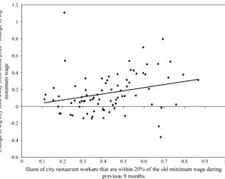
Figure 1 maps each city’s price response to a minimum wage hike against the share of minimum wage workers in the city. Each observation, of which there are 82, represents a city around the time of a minimum wage change. The data cover four federal minimum wage hikes - in 1980, 1981, 1990, and 1991—and a small number of state increases between 1979 and 1995.31 The horizontal axis plots
probðwit¼wmin;itÞ, the share of workers in a city’s restaurant industry that are paid
the minimum wage. This is computed from the outgoing rotation files of the Current Population Survey (CPS). Because employees paid just above the minimum wage are also affected by the law, we include anyone paid within 120 percent of the old min-imum wage during the nine months prior to the minmin-imum wage enactment date. However, the results are not sensitive to picking reasonable thresholds other than 120 percent or time frames other than nine months. The vertical axis displays
Dlnpit
Dlnwmin;it, the ratio of the log change in city food away from home prices to the log
change in the city’s minimum wage. The price data is the CPI for food away from home. The price changes are measured from two months before to two months after the minimum wage is enacted. Dlnpit
Dlnwmin;itis adjusted for year fixed effects to account for
inflation and other secular changes in national labor market conditions.
The most noteworthy aspect of Figure 1 is the positive correlation between the two series. The regression coefficient g is 0.36 with a robust, city clustered-corrected standard error of 0.24.32Not only is the sign of this coefficient consistent with com-petition but the magnitude is as well. Assuming perfect comcom-petition in the labor mar-ket, the regression coefficient should equal labor’s share. Recall from Section III, labor’s share is approximately 30 to 35 percent.
Note also the abundance of observations on Dlnpit
Dlnwmin;it that are positive. Of the 82
city-year observations, 19 are negative, including only two of the largest 30 price responses, defined as when j Dlnpit
Dlnwmin;itj.0:20. These two are interesting in that they
come from the same city, Denver, over consecutive years, 1980 and 1981. Unfortu-nately, we have little information as to what was happening in Denver during this time but we can highlight it for being the main example where city-level prices fall quickly in response to a minimum wage change.33
31. The federal minimum wage increased from $2.90 to $3.10 per hour in January 1980, to $3.35 in Jan-uary 1981, to $3.80 in April 1990, and to $4.25 in April 1991. State increases tend not to occur in states represented by CPI survey cities. The 27 CPI cities are New York City, Philadelphia, Boston, Pittsburgh, Buffalo, Chicago, Detroit, St. Louis, Cleveland, Minneapolis-St. Paul, Milwaukee, Cincinnati, Kansas City, DC, Dallas, Baltimore, Houston, Atlanta, Miami, Los Angeles, San Francisco, Seattle, San Diego, Portland, Honolulu, Anchorage, and Denver. After 1986, prices for 12 of these cities – Buffalo, Minneapolis-St. Paul, Milwaukee, Cincinnati, Kansas City, Atlanta, San Diego, Seattle, Portland, Honolulu, Anchorage, and Den-ver – are reported semiannually. Therefore, we only include pre-1986 observations for these cities. 32. Using the share of minimum wage workers within 110 percent of the old minimum, rather than 120 percent, the point estimate (and adjusted standard error) is 0.42 (0.24). A Huber biweight regression pro-cedure implies a point estimate of 0.28 (0.16) and 0.42 (0.15) using the 110 and 120 percent minimum wage share thresholds. Finally, out of concern that inflation, even over this short period, are driving our results, we tried two things. First, when we include city price deflators as controls on the right hand side, the point estimates are roughly 0.50 with t-statistics of roughly two to 2.5. Alternatively, we look at price changes only over the two months after the minimum wage change. In this case, the point estimate is between 0.20 and 0.30, again with t-statistics of roughly two to 2.5.
33. Because Denver is one of the 12 cities surveyed semiannually starting in 1986, we do not include the 1990 and 1991 Denver data points in the figure. However, they are both positive, albeit small: 0.19 for 1990 and 0.09 for 1991.
The most plausible alternative explanation for these price responses is that they are driven by shocks to demand that happen to be correlated with changes to the mini-mum wage. We tried two ways to test this possibility. First, we estimated Equation 2 without year fixed effects but included changes in the city CPI in thexitvector. The intercept from this specification is not statistically different from zero, suggesting that prices do not rise after minimum wage hikes in areas where the minimum wage does not bind. This finding is consistent with the view that demand shocks are not confounding our estimates because if they were, we would expect that prices would rise in areas where the minimum wage does not bind.
As a second check, we searched for alternative measures ofpitthat vary by local demand conditions, are available for our city panel, and, most importantly, are rela-tively unaffected by low-wage labor costs. By far, the two best candidates are hous-ing and medical care. Therefore, we reran the regression described above, but substituted food away from home prices with these two indices. As expected, we find no evidence that minimum wage hikes are associated with price hikes for housing and medical care.34
Finally, we can compare the estimates in Table 2 to predicted pass-through under competition and constant returns to scale technology using metro variation in
Figure 1
City Level Price Increases
restaurant wage distributions from the outgoing rotation files of the CPS. Under com-petition, the relationship between these predicted price responses and the share of restaurant workers impacted by minimum wage laws should correspond to labor share.
To conduct this test, we define two groups of cities. High wage cities are those with an average hourly wage among the top fifth of all metropolitan areas in 1997–98. Low-wage cities are those with average wages among the bottom fifth of all metropolitan areas in 1997–98. Among high (low) wage cities, 34 (59) percent of all restaurant workers are paid within 120 percent of the minimum wage, our rough measure of the share of workers impacted by such laws. Based on the esti-mates in Column 4 of Table 2, the average predicted price response for low and high wage cities is 0.097 and 0.090, respectively.35The relationship between these vari-ables (slope of the line connecting high and low-wage cities) is :972:90
:592:34¼0:28, slightly lower than, and statistically indistinguishable from, observed labor share in the restaurant industry. Furthermore, we get a similar labor share prediction when we estimate Equation 2 using the store-level data.36
IV. Theory
In this section, we show how our results contribute to the debate on the employment effects of the minimum wage. Assorted models offer differing explanations for why the estimated employment responses to minimum wage hikes are small. As we point out below, however, most of these models imply that prices either do not change or fall in response to a minimum wage hike. Therefore, our results provide evidence against models that have been used to explain the small em-ployment responses found in the minimum wage literature.
Throughout the discussion we assume that all firms are profit maximizers and thus set the level of employment,L, at the point where the marginal cost of the last worker hiredMC(L) is equal to the extra revenue she produces (her marginal revenue prod-uct of labor, or MRP(L)). Appendices A and B contain the formal details of the model.
A. The Competitive Model
We begin by briefly considering the textbook competitive model. If a minimum wage is introduced (or increased) beyond the market-clearing wage in a competitive labor
35. The 20th percentile restaurant wage in the high wage cities is $5.25, compared to $4.82 in the low-wage cities.
36. To derivegfrom the micro data, we use the regression results from Column 4 of Table 2, which gives the relationship between Dlnpit
Dlnwmin;itand the 20th percentile of city market wage. Next, we regress the share of
workers in a city’s restaurant industry that are paid the minimum wage,probðwit¼wmin;itÞ, on the 20th
percentile of that city’s market wage. Using the 27 major CPI cities during 1995 to 1997, the point estimate from this latter regression is probðwit¼wmin;itÞ ¼0:83920:0683wage20it+nit, where wage20it is the
20th percentile of cityi’s wage distribution at timet. From these two regression equations, we can solve
g¼0:24. Ideally, we could precisely estimate Equation 2 using the micro data. Unfortunately, the number of observations in the CPS for individual cities can be small. Consequently,probðwit¼wmin;itÞcannot be
precisely estimated. Butwage20itcan.
market, the marginal cost of hiring a worker increases. In response, holding all else equal, firms will move along their downward-sloping marginal revenue product of labor curve until they reach the point whereMRP(L) is again equated to marginal cost. HigherMRP(L) can only be obtained by reducing the work force. Why? One important reason is that fewer workers imply less output. Even if an additional worker produced the same amount as the previous worker, reduced output increases output prices, marginal revenue, and thus the marginal revenue product of labor. Therefore, minimum wage hikes cause prices to rise and employment to fall in a competitive labor market environment.
B. The Textbook Monopsony Model
However, under monopsony, increasing the minimum wage can cause employment to rise. The fundamental reason is tied to the link between the wage, the marginal cost of labor, and the product price. In this section, we describe the textbook model of monopsony, where firms are monopolists in the product market and monopsonists in the labor market. In Section IVC we show that the key results hold under the more realistic scenario of monopolistic competition in the product market and monopso-nistic competition in the labor market.
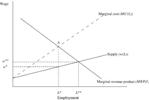
Unlike the competitive firm, which pays the prevailing market wage regardless of how much labor it demands, if the monopsonist wants to expand its labor force, it has to raise the wage of its current workers as well.37Therefore, the marginal cost of hir-ing a worker is greater than the new worker’s wage. Figure 2 shows the wage the firm would have to pay in order to attract an additional worker,w(L), and the marginal cost of hiring that workerMC(L). When the monopsonist maximizes profits by set-ting marginal costs equal to marginal product, shown at pointA, total market em-ployment,L, is lower than the ‘‘competitive case’’ (L) where employment is set based on the prevailing market wagew.
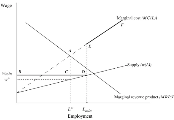
A properly placed minimum wage, set somewhere between the wage paid by a monopsonist (w) and the wage paid by a perfect competitor (w), will increase em-ployment. The intuition for this result, displayed in Figure 3, is that although the minimum wageincreasesthe firm’s average cost of labor, itreducesthe marginal cost of labor. Recall that, absent a minimum wage, the marginal cost of hiring that last worker (at pointA) lies above the wage paid by the monopsonist (because every-one’s wage has to be raised in order to induce a marginal worker to join the firm). If the minimum wage is set above the monopsony equilibrium wage but below the mar-ginal cost of hiring a worker, the new marmar-ginal cost of hiring a worker falls from pointAto pointC (the new marginal cost of labor curve isBCDEF); the marginal cost of hiring additional workers is now just the minimum wage. Because the firm must pay all workers at least the minimum wage, regardless of employment level, the firm does not have to increase the pay of its existing work force to attract more employees (so long as employment is belowLmin). This reduction in the marginal cost of hiring additional labor causes firms to expand output and employment in re-sponse to the minimum wage increase.
Moreover, employment and prices are negatively related because the fall in the marginal cost of labor causes the marginal cost of producing an extra unit to fall. Consequently, the product price falls as well.
It is important to note that if firms are monopsonists in the labor market but the min-imum wage is set sufficiently high (abovewin Figure 2), employment is determined by the intersection of the minimum wage and the marginal product of revenue curve. In this case, an increase in the minimum wage increases prices and reduces employment, just like in a competitive labor market. Thus our empirical results cannot necessarily disprove the existence of monopsony labor markets in cases where the minimum wage is set high (above competitive market-clearing levels). However, we believe our empir-ical results should temper enthusiasm for monopsony power being the explanation for the negligible employment responses found in the literature.
C. Price and Employment Responses When There Is Monopsonistic Competition in the Labor Market and Monopolistic Competition in the Product Market
The results in the previous section were based on a very stylized model. In this sec-tion, we show that those results are quite general under weak assumptions about tech-nology, the product market, and the labor market. Specifically, the results hold when firms have a production function with substitutability between labor and other inputs, monopolistic competition in the product market, and monopsonistic competition in the labor market.
Several researchers have argued that monopsonistic competition in the labor mar-ket is the relevant case (Bhaskar and To 1999; Dickens, Machin, and Manning 1999). That is, workers are not indifferent between employers, even if all employers pay the
Figure 2
Illustration of Monopsony Equilibrium
same wage. One plausible explanation is geography. Employers are located in differ-ent places and transportation costs are large relative to earnings of minimum wage workers. Thus a worker is willing to take a low paying job in order to be relatively near home. Alternatively, teenagers may want to work at the same restaurant as their friends. More generally, certain aspects of one employer may be disagreeable to some workers but not others.
In order to simplify the problem, we make six assumptions beyond the usual axi-oms of firm behavior:
Assumption 1There is a fixed number N of firms.
Assumption 2 All firms have an identical production function, Qn¼QðKn;LnÞ
where Qn;Kn;Lnare output, an aggregator of nonlabor input (that includes capital),
and labor at the nthfirm.
Assumption 3The production function is increasing in all inputs, concave, con-tinuous and twice differentiable.
Assumption 4 K and L are complementary inputs in the production function
ðQ12.0Þ.
Assumption 5 The utility function of the representative consumer is U¼ ðð12aÞQ012h+aQ˜12hÞ
1
12h, where Q0 is the numeraire good, a is close to zero,
˜
Q[ð+Nn¼1Q 12hZ
n Þ
1
12hZ,and Qndenotes output at the nthrestaurant. Concavity implies
h.0andhZ 2 ½0;1Þ.
Figure 3
Assumption 6The firm is a price taker in the capital market and purchases Knat
price r.However, the firm is potentially a monopsonist in the labor market. The
quan-tity of labor supplied to the firm is LSn¼Lðwn;w2nÞ,where w2nis the average wage
paid by all other firms,dLðwn;w2nÞ
dwn jw2n¼wmin.0;and
dLðwn;w2nÞ
dwn jw2n¼wn.0.
Under these assumptions, firms sell their products at a price pðQÞ and choose inputs to maximize profitsp:
pnðKn;LnÞ ¼pðQnÞQn2wnLn2rKn: ð3Þ
These assumptions are standard, although a few require some elaboration. As-sumption 5 gives rise to monopolistic competition in the product market. Markets are perfectly competitive ifhZ¼0 and firms operate as monopolists ifhZ ¼h. As-sumption 6 states that the quantity of labor supplied to the firm need not be perfectly elastic and, therefore, firms face a monopsonistically competitive labor market. Con-sequently, firms face a weakly upward-sloping inverse labor supply curve, wðLnÞ, wheredwðLn;w2nÞ
dLn $0. However, because the minimum wage potentially binds, the
of-fered wage iswn¼maxfwðLn;w2nÞ;wming.38
Firms may be price takers in the labor market because the labor supply curve that the firm faces is perfectly elastic or the minimum wage is sufficiently high that it destroys the firm’s monopsony power. Either way, if firms are price takers in the la-bor market, Theorem 1 holds.
Theorem 1Given the assumptions above, and if firms are price takers in the labor market, the industry level demand curve for labor slopes down.
Proof: see Appendix 1. Theorem 1 is more general than the discussion in Section IVA. There, it is presumed that firms make employment decisions given a fixed
MRP(L) curve, an assumption that is appropriate for monopolists. But, under monop-olistic competition, minimum wage changes potentially shift theMRP(L) curve by altering the decision of other firms, and thus influencing aggregate prices. Theorem 1 also differs from the Weak Axiom of Profit Maximization, which assumes perfect competition in both the product and factor markets.39
Section IVB discusses why employment can rise under monopsony. Given As-sumption 6, this is true under monopolistic competition as well. Together with The-orem 1, this shows that minimum wage hikes cause employment to fall under competition and rise under monopsony.
The next theorem shows that we can use prices to infer the importance of monop-sony power in the labor market.
38. The assumption of capital and labor being complementary inputs (i.e.Q12.0) rules out situations where the profit maximizing choice would be to switch from a capital intensive, high output technology to a labor intensive, low output technology. An example of this is a firm that is capital efficient only up to a certain size. After this size, capital cannot be efficiently used. For example, supposep¼1,r¼1;Q¼K:5L:5ifL
,10 and
Q¼L:5ifL$10. IncreasingLfrom nine to ten would reduce output but depending on the cost of labor, could
increase profits. However, this rather extreme counter-example appears to go against the empirical evidence. For example, it is difficult to reject the hypothesis that production functions are constant returns to scale, and constant returns production functions implicitly assumeQ12.0.
39. See Varian (1984) and Kennan (1998) for proofs of Theorem 1 under competition and monopoly, re-spectively. We have also proved the theorems in this section for the case where firms are Cournot compet-itors in the output market. Proofs are available from the authors.
Theorem 2Given an increase in a binding minimum wage, prices rise under
per-fect competition and, so long as wmin,w,prices fall under monopsony.
Proof: see Appendix 1. The intuition for Theorem 2 was discussed in Section IVB. Finally, there is the quantitative importance of price pass through when there is monopolistic competition in the product market. Theorem 3 shows that if the produc-tion funcproduc-tion is constant elasticity of substituproduc-tion, then firms still push 100 percent of the higher labor costs onto consumers in the form of higher prices.
Theorem 3If Q(.,.)is a constant elasticity of substitution aggregator, and if firms are price takers in the labor market, thenddlnwlnp
min¼minimum wage labor’s share.
Proof: see Aaronson and French (2007). The intuition for this result is straightfor-ward. Given the assumptions above, firms have a constant marginal cost and thus have a horizontal supply curve. Thus, in a perfectly competitive market, all higher labor costs will be pushed onto consumers in the form of higher prices. In the case of monopolistic competition in the product market, there is a constant markup over marginal cost. Thus the supply curve is still horizontal and all labor costs are pushed onto consumers in the form of higher prices.
Furthermore, Aaronson and French give predicted price and employment responses under monopsonistic competition. They show that if the employment re-sponse is large and positive, then the price rere-sponse will be large and negative. For example, if the employment elasticity is +0.2, which is possible under monop-sony, then the price response will be -0.05. These price responses vary notably from what is reported in Table 2.
The only assumption that we view as not innocuous is the first. Although the size of a business is allowed to change in response to a higher minimum wage, firm exit or entry is precluded. We think this is a reasonable assumption given the existing, albeit rather meager, empirical evidence.40Moreover, in this paper, we are interested in a short-term response that likely severely limits entry and exit decisions.
The main reason for assuming no exit is that under monopsony, minimum wage hikes increase employment per restaurant, but likely reduce the total number of restaurants. Therefore, the industry level employment response is ambiguous. In this sense, we view the assumption of no exit as supporting the monopsony argument.41
40. Card and Krueger (1995) and Machin and Wilson (2004) find no effect in the U.S. and U.K., respec-tively. We have done some analysis of restaurant entry and exit using the Census’ Longitudinal Business Database. Consistent with the literature, our preliminary findings suggest negligible entry and exit effects in the year following a minimum wage change. These results stand in contrast to those of Campbell and Lapham (2004), who find a significant amount of retail net entry along the U.S.-Canada border within a year of exchange rate movements. We suspect these different results reflect the importance of exchange rates relative to minimum wage levels in terms of firm costs.
D. Efficiency Wage Models
Efficiency wage models (where increased wages increase effort or reduce turnover costs), often give monopsy-like predictions. Manning (1995), Rebitzer and Taylor (1995), and Deltas (2007) all present models where increases in the minimum wage can increase employment. None of these models allows for capital-labor substitut-ability, and only Deltas (2007) allows for endogenous prices. Below we present an efficiency wage model with endogenous prices and capital-labor substitutability.
We follow Solow (1979), who argues that the wage affects morale and effort amongst other things, and let the wage enter the production function directly. If an increase in the wage causes increased effort, more meals can be produced with the same amount of labor and capital. Therefore, it is not necessarily more costly to pro-duce meals when the minimum wage increases. This can attenuate the disemploy-ment effects of the minimum wage. However, if employdisemploy-ment does not fall (and other factors do not fall either) and productivity rises, total output will rise and prod-uct prices will fall.
Let the production function be:
Q¼QðK;L;wÞ ¼ ðð12aÞKr+aðLwuÞrÞ1r;
ð4Þ
wheres[121ris the partial elasticity of substitution betweenKandLw
uin the
pro-duction ofQ, andLwuis ‘‘effective labor.’’ The parameter 0# u,1 may be greater than 0 because increases in the wage increase effort, which could happen for a vari-ety of reasons. Furthermore, assume that Assumptions 1 to 5 in Section IVC hold. Then the price and employment responses are:
dlnp
dlnw¼sð12uÞ
ð5Þ
dlnL
dlnw¼2ð12uÞðð12sÞs2shÞ2u
ð6Þ
wheresis the share of total costs going to labor. Whenu¼0, Equations 5 and 6 give the textbook response to the minimum wage. However, whenu.0 (and all else is equal), a one percent increase in the wage increases effective laborupercent, causing the marginal cost of effective labor to only rise 12upercent. This has implications for both prices and employment responses. The price response is attenuated, rising by sð12uÞ percent, a fraction ð12uÞ less than without endogenous work effort. The employment response is also muted byð12uÞdue to an increase in the marginal cost of labor. However, the same amount of effective labor and output can be pro-duced with fewer bodies, lessening the need for labor (the 2uterm at the end of Equation 6).
Regardless, while a smaller employment response relative to the case without en-dogenous work effort is possible, the model clearly predicts a smaller price response as well. However, our estimates indicate large price responses to the minimum wage. Thus, our price results provide evidence against the hypothesis that endogenous work effort is responsible for the small observed employment responses to minimum wage hikes.
E. Other Models of the Employment Effects of the Minimum Wage
We have argued that the price responses to minimum wage hikes are useful for dis-tinguishing between competition and monopsony in the labor market. Likewise, our estimated price responses help shed light on other explanations of the small employ-ment response found in the minimum wage literature.
Some researchers (for example, Kennan 1995; MaCurdy and O’Brien-Strain 2000) suggest higher income resulting from a minimum wage increase causes low-wage workers to buy more minimum wage products, attenuating the disemployment effect of the minimum wage. For the restaurant industry, Kennan refers to this possibility as the ‘‘hungry teenager hypothesis.’’ The price response reported in this paper is a key parameter for such a calculation. Aaronson and French (2006) write down a model that allows for such demand-induced feedbacks and show that increases in the min-imum wage reduce real income for nonminmin-imum wage workers (because prices rise) but increase real income of minimum wage workers (because their wage rises). They find that if minimum wage workers spend a large fraction of their income on fast food, then the rise in incomes for fast food workers can at least partly offset the dis-employment effect of the minimum wage. Using data from the Consumer Expendi-ture Survey and U.S. Department of AgriculExpendi-ture’s Continuing Survey of Food Intake by Individuals, they find that minimum wage workers spend between 20 and 100 per-cent more of their income on fast food as those who are not minimum wage work-ers.42Given these estimates (and other calibrated parameters) the increased income going to minimum wage workers can offset between 25 and 40 percent of the output loss, and 10 to 30 percent of the employment loss of a model that does not account for the increased income and increased expenditures of minimum wage workers.
Our price responses are less consistent with the idea that that minimum wage laws merely cause firms to reshuffle compensation packages from nonwage benefits to wages. For example, fast food restaurants could stop giving workers free meals after minimum wage hikes. Hashimoto (1982) and Neumark and Wascher (2001) argue that firms may reduce training after minimum wage hikes. As a result, there is no increase in the cost of labor faced by firms. However, if the minimum wage does not increase the cost of labor, it is unclear why there are price increases after minimum wage changes. Although shifting compensation packages from nonwage to wage benefits may occur, our results indicate that firms still bear a sizeable fraction of the cost of minimum wage hikes. In this sense, our findings are consistent with Card and Krueger (1995), who also find very little substitution between wage and nonwage benefits after minimum wage hikes and also find no evidence of minimum wage hikes on training. Finally, our analysis has not considered search models (for example, Burdett and Mortensen 1998), which also give monopsony implications for employment. A full analysis of the variety of search models is well beyond the scope of this paper, es-pecially because most of them would need to be modified to account for endogenous product prices and capital labor substituability. However, it seems likely that employ-ment and prices would move in opposite directions in most standard applications of search. For example, given that the Burdett and Mortensen production technology is
linear in labor (that is, no substitution among inputs), increases in employment in-crease output and should presumably reduce the product price were it endogenized. It is also worth noting that most estimated search models, including Van den Berg and Ridder (1998), Flinn (2006), Ahn and Arcidiacono (2003), find some disemploy-ment in response to a minimum wage increase.
Arguably, our empirical results themselves—that marginal cost shocks are passed onto consumers through higher output prices—may be consistent with small disem-ployment effects. If restaurants face factors that limit their ability to raise prices, say because it is costly to switch prices, or because the price elasticity of demand for food away from home is infinitely elastic, the predicted disemployment effects of a minimum wage increase would be larger than if these factors did not hinder price behavior. If firms cannot pass cost increases onto consumers, then profits will be squeezed and firms may sharply cut their work force. Given that we find rather large price increases in response to minimum wage hikes, firms seem to be able to push costs onto consumers, and are not having their profits greatly reduced.
Instead, we interpret our results to be consistent with the moderate disemployment effects reported in Aaronson and French (2007). They calibrate a structural model of labor demand that incorporates the price responses found here to show that a 10 per-cent increase in the minimum wage reduces restaurant employment by 2 to 3 perper-cent, a short-run response that is within the range of estimates found in the literature. Moreover, the total (low plus high skill) restaurant employment response may be as small as 1 percent.
V. Conclusion
Much work has looked at the employment implications of raising the minimum wage, with a range of estimates reported in the literature. We offer new em-pirical evidence using output prices both at the store-level and aggregated to the city-level. In both cases, prices unambiguously increase in response to a minimum wage change. Furthermore, the results are similar across three sources of variation in the data: cross-state differences in the size of the minimum wage change, cross-restaurant type differences in the tendency to pay at or near the minimum wage, and cross-metro differ-ences in the fraction of workers paid at or near the minimum wage. There is no evidence that prices fall in response to a minimum wage increase.