Full Terms & Conditions of access and use can be found at
http://www.tandfonline.com/action/journalInformation?journalCode=ubes20
Download by: [Universitas Maritim Raja Ali Haji] Date: 12 January 2016, At: 17:41
Journal of Business & Economic Statistics
ISSN: 0735-0015 (Print) 1537-2707 (Online) Journal homepage: http://www.tandfonline.com/loi/ubes20
Binomial Autoregressive Moving Average Models
With an Application to U.S. Recessions
Richard Startz
To cite this article: Richard Startz (2008) Binomial Autoregressive Moving Average Models With an Application to U.S. Recessions, Journal of Business & Economic Statistics, 26:1, 1-8, DOI: 10.1198/073500107000000151
To link to this article: http://dx.doi.org/10.1198/073500107000000151
Published online: 01 Jan 2012.
Submit your article to this journal
Article views: 149
View related articles
Binomial Autoregressive Moving Average
Models With an Application to U.S. Recessions
Richard S
TARTZDepartment of Economics, University of Washington, Seattle, WA 98195 (startz@u.washington.edu) Binary Autoregressive Moving Average (BARMA) models provide a modeling technology for binary time series analogous to the classic Gaussian ARMA models used for continuous data. BARMA models mitigate the curse of dimensionality found in long lag Markov models and allow for non-Markovian persistence. The autopersistence function (APF) and autopersistence graph (APG) provide analogs to the autocorrelation function and correlogram. Parameters of the BARMA model may be estimated by either maximum likelihood or MCMC methods. Application of the BARMA model to U.S. recession data suggests that a BARMA(2,2) model is superior to traditional Markov models.
KEY WORDS: ARMA models; Binary variables; Markov models; Time series.
1. INTRODUCTION
Binary time series are typically modeled in economics as Markov processes, most often as first-order Markov processes. In contrast, for continuous-valued time series, the Gaussian autoregressive-moving average model is widely used. This sit-uation persists despite the introduction in the statistics litera-ture of several ARMA models for discrete variables. (An early paper is Jacobs and Lewis 1978. See Benjamin, Rigby, and Stasinopoulos 2003 for the introduction of GARMA models, as well as a review of the literature.) In this article I suggest a new practical tool for analysis of binary series: the autoper-sistence function and autoperautoper-sistence graph, analogous to the standard autocorrelation function and correlogram. I then turn to remarks on Li’s (1994) elegant, but too little used, binary au-toregressive moving average (BARMA) model. Parameters of the BARMA model may be estimated either by maximum like-lihood or, as I show below, by MCMC methods. These tools are used to analyze quarterly data on U.S. recessions, which are seen to be non-Markovian.
Although an obviously valuable tool for the study of binary time series, Markov models suffer from two practical shortcom-ings. First, they do not fit well when data have strong moving average components. Second, when there are long lags, Markov models face the curse of dimensionality. Whereas the models discussed later can include Markov models as special cases, they would typically be more general in that they add in a mov-ing average component. These models also provide a conve-nient way to place restrictions on the pure Markov models to eliminate the curse of dimensionality.
The study of Gaussian ARMA models traditionally starts with an identification step in which the correlogram is examined to suggest a model whose ARMA representation is estimated in the next step. Correlation is a natural metric for a Gaussian se-ries, but much less so for a binary series. Obversely, looking at a conditional probability is more natural for a binary than for a continuous series, since a binary series has only two dis-crete values on which it is necessary to condition. After defin-ing tools for the identification step for binary data, I apply them to U.S. recessions. The Binary Autoregressive (BAR) model is discussed as a way to connect BARMA models with Markov models. After I discuss several practical difficulties, I then ap-ply the full BARMA model to the recession data.
2. THE AUTOPERSISTENCE FUNCTION
The autocorrelation function and correlogram provide use-ful information about the behavior of theoretical and empirical continuous time series. Analogously, the autopersistence func-tion and autopersistence graph provide useful informafunc-tion about the behavior of theoretical and empirical binary time series.
2.1 ACF, Correlogram, APF, and APG
For a stationary, ergodic,Gaussian ARMA(p,q)process, the joint distribution of the observations is completely described by the autocorrelation function, ACF (together with the uncondi-tional mean and variance). Similarly, an observed series is de-scribed by its correlogram. The ACF and correlogram are useful for continuous data even when the time series is not Gaussian. The shape of the correlogram sometimes provides a hint as to the order of the underlying ARMA process, whereasACF(k)is informative about how quickly information in the current obser-vation fades in a given theoretical process. The ACF or correlo-gram provides the information necessary for making ak-ahead linear forecast from the current observation on the series. For a first-order autoregressive series, theAR(1)parameter is esti-mated byACF(1)and the shape of the ACF follows a familiar geometric decline asymptoting to zero.
Looking at correlations is less useful as a summary statis-tic for a binary series than it is for continuous series. However, looking atk-ahead conditional probabilities is useful and is fea-sible since one need only condition on two values rather than on a continuum.
For an ergodic, binary time seriesy, where w.o.l.g.ytakes the values 0 and 1, the appropriate analog to the ACF is the pair of autopersistence functions,APF0(k)≡Pr(yt+k=1|yt=0)and
APF1(k)≡Pr(yt+k =1|yt =1). The autopersistence graphs
APG0 andAPG1 are, by analogy to the correlogram, the em-pirical counterparts to the APF and may be estimated by the appropriate sample conditional means. Whereas the APF does not completely describe the joint distribution of an ergodic se-ries (nor does the ACF for a continuous sese-ries except in the
© 2008 American Statistical Association Journal of Business & Economic Statistics January 2008, Vol. 26, No. 1 DOI 10.1198/073500107000000151
1
2 Journal of Business & Economic Statistics, January 2008
Gaussian case), the shape of the APG may provide a hint about the order of an appropriate BARMA process.APF(k)is infor-mative about how quickly information in the current observa-tion fades. The APF or APG provides the informaobserva-tion necessary for making ak-ahead forecast from the current observation on the series (although the APF is more limited than the Gaussian ACF in that the APF can be used to forecast conditional only on the current observation, whereas in the Gaussian case the ACF can be used to predict conditionally on any set of lags). For a first-order Markov process the two transition probabilities are estimated byAPF0(1)andAPF1(1), and the shape of the APF follows a familiar geometric decline asymptoting to the uncon-ditional mean.
2.2 U.S. Recession Data
Figure 1 shows the APG for U.S. recessions. The oscillating nature of the APG, being very unlike a geometric decline, sug-gests that a first-order Markov is not a good model for these data. With this as a motivating example, I begin with theory and then return to an empirical examination of recession data in Section 8.
3. BINARY AUTOREGRESSIVE MODELS
For what follows, it is useful to recast thepth-order Markov model in an autoregressive framework. The Binary Autoregres-sive with Cross-terms model of orderp,BARX(p), suggested by Zeger and Qaqish (1988), can be written
ηt=β0+Ip≥1
whereIp≥i is the indicator function. In other words, the model
includes all the unique lags and lagged cross-terms through lagp. The log-likelihood equals
£=
The BARX(p)model is an alternative representation of the pth-order Markov model and one can map back and forth between the parameters of the BARX and the Markov represen-tations. The BARX approach has two minor disadvantages rel-ative to the familiarMarkov(p)representation: transition prob-abilities on the edge of the parameter space, 0 or 1, require infinite values for the BARX parameters, and the interpretation ofβ0and−→φ is less familiar than direct statement of the tran-sition probabilities. The advantage of the BARX representation is that it provides a natural starting point for moving away from unrestricted Markov models.
Figure 1. Persistence of U.S. recessions. ( APG0; APG1; mean.)
The difficulty with application of the pth-order Markov model is that it requires 2pparameters to captureplags of be-havior, which is impractical for even modest sizes ofp. As a remedy, Raftery (1985) suggested the Mixture Transition Dis-tribution model to impose linear restrictions on the Markov transition probabilities to reduce the size of the parameter space from 2ptop. Similarly, the Binary Autoregressive model of or-derp(first suggested by Cox 1981),BAR(p), imposes linear re-strictions on theBARX(p)model in the form of zero restrictions on cross-terms, substituting
ηt=β0+φ1yt−1+φ2yt−2+ · · · +φpyt−p. (3)
In the BAR model, restrictions are linear in logits of the transition probabilities rather than in the transition probabil-ities themselves. Models intermediate between BAR(p) and BARX(p)may be specified in a natural way, for example by including cross-pairs but not cross-triples or higher.
Use of the logit link function,µt= e ηt
1+eηt, is convenient, but a
different link function could also be used. For example, a stan-dard normal CDF would lead to a probit-based model. Eichen-green, Watson, and Grossman (1985) presented a dynamic ordered-probit model for trinary rather than binary outcomes with a somewhat different stochastic specification. de Jong and Woutersen (2005) examined the asymptotic properties of esti-mates of related models.
4. BINARY AUTOREGRESSIVE MOVING
AVERAGE MODELS
Markov models do not give an adequate representation of the persistence of recessions. The APG in Figure 1 crosses the un-conditional mean approximately one year out, and then shows damped, but considerable, oscillation. Whereas a second-order Markov model could in principle produce oscillations in the APF, that does not happen at our estimated parameters (see be-low). This suggests considering non-Markovian models.
Li (1994) suggested formulating theBARMA(p,q)model as
a continuous ARMA model. The BARMA model can be ex-tended by adding cross-terms as in the BARX model above and/or by Li’s suggestion of replacingβ0with a covariates term Xtβ. The moving average component is in the class described
by Cox (1981) as observation-driven. Note that the analogy with the continuous ARMA model is not perfect, because it is the memory of prediction errors (yt−i−E(yt−i)) rather than
shocks that is carried forward.
The BARMA(p,q) model can be estimated by quasi-maxi-mum likelihood. Li suggested setting the initialqvalues ofµtto
zero or to the sample mean ofy. One could also set initial values ofµtto .5 or initial values ofyt−µt to zero. (The estimates in
this article use the sample mean ofyfor initial values ofµt.)
5. PRACTICAL CONSIDERATIONS
I turn now to some practical considerations in the use of the BARMA model, as illustrated with the recession data.
5.1 Three Practical Considerations for the BAR Model
Parameterization of the BAR in terms of logits on transition probabilities raises three practical considerations, each of which arises with the sample data. The first issue is what happens when the estimated parameters are on the edge of the permissi-ble space. For my recession data, the transition probabilities for a second-order Markov are
Pr(yt=1|yt−2,yt−1)= .
090141 0
1 .824176 , so two of the four parameters take limiting values. The BARX(2) representation is β0= −2.49268, φ1= ∞, φ2 =
−∞,φ12=4.03758. Estimation of theBARX(2)represents no difficulty, as large values ofφare effectively infinite, as long as the user remembers thatφ=25 andφ=2,500 mean the same thing. Likelihood values are computed correctly.
The second practical issue that can arise is dealing with empty cell counts. For example, despite having 600 observa-tions for our recession data, the eight sample transition prob-abilities for a third-order Markov process produce two empty cells (plus, as it happens, four cells with 0 or 1 probabilities and two interior values). Therefore, some parameters in the Markov(3)/BARX(3)representation are unidentified. Although this does not prevent calculation of the likelihood function, use of a likelihood value based on unidentified parameters for test-ing may be unwise. Furthermore, havtest-ing unidentified parame-ters is problematic in analysis and simulation of the estimated process, because these require values for the cells that were unobserved in the sample. The linear restrictions implicit in the BAR model reduce the information required for parame-ter identification so that the BAR model is generally unaffected by the presence of empty cells. As it happens, my data have a BAR(3)representation with an identical likelihood value as the third-order Markov.
The third practical consideration regards both calculation of Wald statistics and the behavior of search algorithms when pa-rameters are on the edge of the permissible space. Both issues require looking at the second partials of the log-likelihood func-tion, computation of which can be problematic. For theBAR(p)
model, the observation-by-observation contributions to the sec-ond partials forβ0,φ1, andφ2are
nal element in the second-partials matrix equals zero. When yt−1=0, the second diagonal element equals zero as well. As a result, the estimated information matrix is singular. It follows that the traditional estimates of the variance–covariance ma-trix of the parameters is unavailable, as are the associated Wald tests.
Having a singular information matrix when the maximum likelihood estimate ofφ1is large may be regarded as a desir-able feature. Since the MLE parameter estimates do not follow the standard distributions at the edge of the permissible para-meter space, variance estimates and Wald tests may well be misleading. However, the estimated log-likelihood is also flat for extreme values of φ examined in the search process even though these values are very far from the MLE. As a result, standard search algorithms that rely on second partials can be-come “stuck” in areas of the parameter space far from the op-timum. Modification of such algorithms or manual intervention in the search process may be needed. When φ1 is close to a global maximum, this suggests that an arbitrary scaling can be applied to the parameter set, soφ1should be set to a large con-stant (e.g., φ1=100) and the search should continue for the remaining parameters. (I am grateful to Jim Hamilton for this suggestion.) Alternatively, use of the Gibbs sampler proposed in Section 7 avoids numerical problems with the likelihood func-tion entirely.
5.2 Practical Analysis of the BARMA and BMA Models
Unlike the Gaussian ARMA model, the BARMA model is inherently nonlinear, and does not directly translate between AR and MA representations. Because of the logit link, there are no pleasant analytic solutions for the APF, autocorrelations, or even the unconditional mean.
Whereas a BAR(p)model always has a pth-order Markov representation, for which there are a variety of tools available, a model with a BMA component does not. Fortunately, given the recursive nature of the BARMA specification, the APF and so on can be drawn by straightforward numerical simulation, start-ing at arbitrary initial values, discardstart-ing the first few draws, and then using simulation sample averages for the desired statistic. Such a simulation assumes that the process does not have an absorbing state. In economics this is not an issue, as the usual assumption is that we are sampling from a time series process
4 Journal of Business & Economic Statistics, January 2008
with a very long history, implying that if the process has an ab-sorbing state, our entire sample will be in the abab-sorbing state. In other areas the issue of an absorbing state may be more prob-lematic.
Interpretation of magnitudes for BARMA coefficients is less neat than for Gaussian ARMA models, but some examples pro-vide intuition. A BARMA coefficient gives the change in the log odds ratio when the corresponding data lag equals 1 rather than 0. For a BAR(1) with β0=0, for example, observing from.9 to.999. This suggests as a rule of thumb that BARMA coefficients above 1 are “large” and coefficients in the high sin-gle digits are very large.
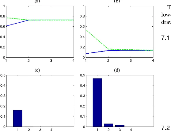
The APF for a BMA(q)model returns to the unconditional mean (and the autocorrelation function goes to zero after q lags)—almost. Because of the curvature of the logit function, theAPF(k)fork>qcan differ very slightly from the uncondi-tional mean. Consider Li’s simulation of aBMA(1)with para-metersβ0=1 andθ1=.8, for which he stated “insignificant autocorrelations after lag one. . . are typical.” The left panel of Figure 2 shows the APF and autocorrelation function (for 2,000 simulations) for Li’s parameters, confirming his claims. As a contrast, the right panel shows the APF and autocorrelation function forβ0= −2.2 andθ1=4.4. The unconditional expec-tation of yis .136. The first two values of APF1 are .539 and .160; soAPF1(2)is measurably above the unconditional expec-tation. Similarly,ACF(2)=.028, which is not quite zero. Thus, while pure BMA models do not formally have the same finite autocorrelation function property found for Gaussian models, the deviation is so small as to be unlikely to have much practi-cal consequence.
(a) (b)
(c) (d)
Figure 2. (a)BARMA(0,1)APFβ0=1,θ=.8; (b)BARMA(0,1)
APFβ0=2.2, θ=4.4; (c) BARMA(0,1)autocorrelation function; (d)BARMA(0,1)autocorrelation function.
6. GOODNESS–OF–FIT MEASURES
Comparison of a model’s APF with the empirical APG is one way to evaluate model adequacy. Scalar goodness-of-fit measures are also useful. One obvious measure is McFadden’s (1974)R2M≡1−£/£0, where£ is the maximized model log-likelihood and £0 is the restricted log-likelihood from maxi-mizing ηt =β0, in other words from simply using the sam-ple mean. Another measure is thepredictive R2p≡1−(yt−
µt)2/(yt− ¯µ)2, whereµ¯ is the sample mean, due to Efron
(1978). If one’s interest is forecasting and one has a mean square error loss function, thenR2pis the appropriate in-sample goodness-of-fit measure.
7. GIBBS SAMPLING
Estimation of the BARMA model by Gibbs sampling makes available the set of tools associated with MCMC methods. Ad-ditionally, Gibbs sampling avoids the computational issues de-scribed earlier. The approach here is similar to Gibbs sampling for probits. (See Albert and Chib 1993 or the expository pre-sentation in Koop 2003.) The model is augmented with a la-tent variableη∗, and sampling proceeds in three blocks. In the first block,η∗ is effectively regressed on the right side of the BARMA model to draw the BARMA parameters. Here, a dif-fuse prior is assumed. Any prior applicable to a regression could be used. In the second block, values ofµ∗are drawn (condition-ally deterministic(condition-ally) by evaluating the BARMA model. In the third block, the latentη∗are drawn from truncated logits.
To motivate the latent variable model, assume that nature drawszt∼uniform(0,1)andyt=1 iffµt>zt.This is
equiv-alent tog−1(µt) >g−1(zt), whereg= e ηt
1+eηt. Define the latent
variableη∗t =g−1(µt)−g−1(zt), so thatyt=1 iffη∗t >0.One
can then rewrite the BARMA equation as a linear regression:
η∗t =β0+
The Gibbs sampler consists of an initialization block fol-lowed by iteration between drawing regression coefficients, drawingµ∗, and drawingη∗.
Discarding the first max(p,q)observations, create X where the first column equals 1.0, followed byp columns of lags of y,followed byqcolumns ofy−µ∗:
˜
b∼N
(X′X)−1X′η∗,π
2 3 (X
′X)−1
, (8)
β0= ˜b0,
φ= ˜b1,...,p,
θ= ˜bp+1,...,q.
I treat the posterior for the regression parameters as multi-variate normal, even though the errors are logistic rather than normal. (I am grateful to Michael Dueker for pointing out that this can be regarded as a draw from a proposal density in a Metropolis–Hastings step.)
Note that (8) assumes a diffuse prior for the BARMA para-meters. Since the variance of the logistic distribution is π32, no priors are needed for the regression variance.
7.3 Drawµ∗
Starting att=1+max(p,q), drawη¯t=β0+pi=1φiyt−i+ q
i=1θi(yt−i −µ
∗
t−i), compute µ∗t = e ¯ ηt
1+eη¯t, and proceed
it-eratively. Because of the “observation-driven” nature of the BARMA model, this draw is, conditional on the most recent draw of the BARMA parameters, deterministic.
7.4 Draw Latentη∗
Let FR(η)¯ be the logistic distribution with mean η¯ right-truncated at zero and let FL(η)¯ be the corresponding left-truncated distribution. Draw the latentη∗t according to
η∗t ∼
FR(η¯t) ifyt=0
FL(η¯t) ifyt=1.
(9)
The regression draw, calculation of µ∗, and latent draw blocks are repeated until a sufficient size sample is collected.
8. APPLICATION TO U.S. RECESSIONS
Recessions in the United States are identified by the Busi-ness Cycle Dating Committee of the National Bureau of Eco-nomic Research (NBER). “A recession is a significant decline in economic activity spread across the economy, lasting more than a few months, normally visible in real GDP, real income, employment, industrial production, and wholesale-retail sales” (NBER Business Cycle Dating Committee, October 21, 2003 statement). The NBER identifies 32 recessions since 1854, the shortest being 6 months in length and the longest being 65 months.
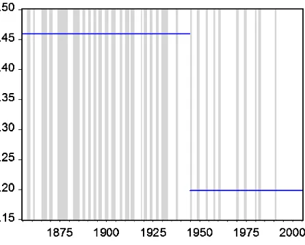
Figure 3 shows the 602 quarterly observations given in the NBER recession chronology, with recession periods shown by shaded areas. In addition, horizontal lines are drawn showing
Figure 3. NBER recession dating ( mean).
the mean probability of the United States being in recession through 1945, and then, separately, in the postwar period. While the NBER dates recessions on a monthly basis, quarterly data are used here. (By convention, a quarter is coded with a 1 for recession if any month in the quarter is identified by the NBER as being in a recession.) This is done for two reasons. First, as most national income accounting data are quarterly, particularly GDP, much statistical modeling of recessions is quarterly. Sec-ond, the notion that recessions last “more than a few months” is typically interpreted as a 6-month minimum, so a monthly se-ries is necessarily difficult to fit well with a low-order Markov model.
Starting from a standard first-order Markov model as a benchmark, we see what extra light can be shed by turning to BAR and BARMA models of recessions.
8.1 Autoregressive Recession Models
The natural starting point for analysis of the time series of U.S. recessions is with a Markov model. (See Hamilton 1989.) Table 1 shows the transition probabilities foryt=1 conditional
on laggedyfor Markov models of order 0 through 3.
The first-order Markov model is clearly preferred to a con-stant mean. The second-order Markov model has a much higher log-likelihood than does the first-order Markov. Note that two of the parameters in the second-order model are on the edge of the parameter space. The third-order Markov model has a yet higher log-likelihood. Note that four of the eight parameters are 0 or 1 and, more problematically, two of the parameters are not identified.
Moving from low-order to higher order Markov models im-proves the log-likelihood function. However, neither of theR2 goodness-of-fit measures is very much improved. Furthermore,
Table 1. Markov models of U.S. recessions
P(yt|(yt−1,yt−2,yt−3)) (0,0,0) (0,0,1) (0,1,0) (0,1,1) (1,0,0) (1,0,1) (1,1,0) (1,1,1) logL R2M R2p
Third-order Markov .0994 0 NA 0 1.0 NA 1.0 .7867 −181.99 .53 .61
Second-order Markov .0901 0 1.0 .8242 −192.05 .51 .60
First-order Markov .0829 .8505 −200.60 .49 .59
Mean .3567 −390.89 0 0
6 Journal of Business & Economic Statistics, January 2008
(a)
(b)
Figure 4. (a) 1st order Markov persistence of U.S. recessions; (b) 2st order Markov persistence of US recessions.
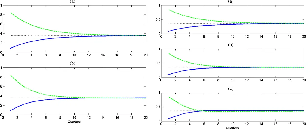
the APF’s for the first- and second-order models are quite sim-ilar to one another (Fig. 4) and not at all like the empirical APG shown in Figure 1. (Note that the APF for the third-order Markov model cannot be calculated since some of the parame-ters are unknown. Here, and in Figures 5–7 and 9,APF1appears with a dashed line,APF0with a solid line, and the steady-state mean with a dotted line.)
The results for the Markov models hint that longer lags matter, but that 600 observations is insufficient to estimate a high-order Markov model. Figure 5 shows the APF’s for BAR(1),BAR(2), andBAR(3)models.BAR(1)and first-order Markov models are necessarily the same. Coincidentally, the four-parameter second-order Markov can be represented ex-actly by a three-parameterBAR(2)(β0= −2.31,φ1=α,φ2=
−α+3.86, for any very large value of α), so for these data the two are equivalent. Serendipitously (all its parameters are identified), the four-parameter BAR(3)(β0= −2.20, φ1=α,
φ2=0,φ3= −α+3.51, for largeα) has the same log likeli-hood value as the eight-parameter third-order Markov model. TheBAR(3)APF returns to the unconditional mean somewhat faster than do the lower order models and shows a shade of the APF crossing property that is prominent in the empirical APG.
8.2 BARMA Recession Models
Can we find a parsimonious BARMA model for understand-ing recessions that improves on the Markov models? Since it is clear from the APG that some autoregressive component exists, pure BMA models are not useful candidates. We present three low-order BARMA models here, as shown in Table 2. The
log-(a)
(b)
(c)
Figure 5. (a)BAR(1) persistence of U.S. recessions; (b)BAR(2)
persistence of U.S. recessions; (c)BAR(3)persistence of U.S. reces-sions.
likelihood of theBARMA(1,1)model is noticeably larger than the log-likelihood of the nestedBARMA(1,0)model, that is, the first-order Markov model shown in Table 1. The same is true in comparingBARMA(2,1)toBARMA(2,0).Figure 6 displays two APF’s. TheBARMA(1,1)APF looks pretty much like the BARMA(1,0)APF. However, whileR2M shows little difference between the BAR and BARMA models,R2pis notably lower for the BARMA models.
TheBARMA(2,2)model has essentially the same likelihood value,R2M, andR2p, as the third-order Markov/BAR(3)model. Figure 7 shows theBARMA(2,2)APF next to the empirical APG. The match is closer than for earlier models. Based on the slightly higher likelihood value for theBARMA(2,2)model and the better match of the APF to the APG, the BARMA model is clearly preferred to an unrestricted Markov model, and arguably to the restrictedBAR(3)as well.
It is unknown whether methods of lag length determina-tion employed for Gaussian ARMA models work well for BARMA models. For the record, the likelihood ratio statistic forBARMA(2,2)versusBARMA(2,4)equals 4.97, which cor-responds to ap-value of .08.
8.3 Gibbs Sampling
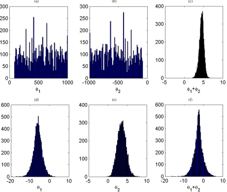
A BARMA(2,2)model was estimated by Gibbs sampling, discarding 1,000 draws and retaining 10,000. Note that the maximum likelihood estimates in Table 2 show effectively in-finite values for both the BAR coefficients withφ1+φ2≈5.0. Figure 8 presents posterior medians and histograms. The results
Table 2. BARMA models of U.S. recessions
β0 φ1 φ2 θ1 θ2 logL R2M R2p
BARMA(2,2) −2.62 42.54 −37.58 −9.53 5.20 −180.78 .54 .61
BARMA(2,1) −2.67 18.84 −13.95 −4.51 −187.53 .52 .27
BARMA(1,1) −2.183 3.53 2.13 −195.94 .50 .24
(a)
(b)
Figure 6. (a) BARMA(1,1) persistence of U.S. recessions; (b)BARMA(2,1)persistence of U.S. recessions.
(a)
(b)
Figure 7. (a) Empirical persistence of U.S. recessions;
(b)BARMA(2,2)persistence of U.S. recessions.
(a) (b) (c)
(d) (e) (f)
Figure 8. (a) median(φ1)= 595.3341; (b) median(φ2)= −590.3878; (c) median(φ1+φ2)=4.5111; (d) median(θ1)= −6.096;
(e)median(θ2)=3.4897; (f)median(θ1+θ2)= −2.6004.
8 Journal of Business & Economic Statistics, January 2008
Table 3. BARMA(2,2)models of U.S. recessions
BARMA(2,2) β0 φ1 φ2 θ1 θ2 logL R2M R2p
All −2.62 42.54 −37.58 −9.53 5.20 −180.78 .54 .61
Pre-1945 −2.64 24.30 −19.06 −10.46 4.50 −114.52 .54 .55
1945– −2.97 24.65 −20.10 −7.12 3.30 −56.20 .54 .61
of the Gibbs sampler are quite close to the MLE results. The BAR coefficients are effectively infinite. Note that the median of φ1+φ2 is close to the MLE estimate and clearly positive. The distribution ofθ1is almost entirely to the left of zero and the distribution ofθ2is almost entirely to the right. The poste-rior forθ1+θ2has greater spread and the median is somewhat farther from the MLE.
8.4 Structural Break in the Recession Process
From visual inspection of Figure 3 it appears that prewar and postwar business cycles are different. (The choice of 1945 as a break date reflects the NBER’s use of 1945 as a break in pre-senting summary statistics.) Since the end of World War II, the U.S. economy has spent a lower proportion of time in reces-sions. Contractions have been shorter and expansions have been longer.
The likelihood ratio statistic on the null of no break equals 20.12, with an associatedp-value of .001. Figure 9 shows the separate APF’s. The shapes change modestly, with the primary difference being the lower postwar mean reflecting the lower value ofβ0.
9. CONCLUSION
TheBARMA(2,2)model is a substantial improvement over the traditional Markov model for U.S. recession data. More
(a)
(b)
Figure 9. (a)BARMA(2,2)pre-1945; (b)BARMA(2,2)1945–.
generally, the BARMA model is a useful extension to the statis-tical toolbox for modeling binary series over time. Its principal advantages are the ability to estimate restricted Markov mod-els to circumvent the curse of dimensionality, and the ability to model non-Markovian processes. The autopersistence function and autopersistence graph provide graphical tools analogous to the autocorrelation function and correlogram used for Gaussian ARMA models.
ACKNOWLEDGMENT
Advice from Peter Hoff, Chang-Jin Kim, Adrian Raftery, Shelly Lundberg, Jim Hamilton (associate editor), and Michael Dueker (the referee) is gratefully acknowledged, as is research support from the Cecil and Jane Castor Professorship at the University of Washington.
[Received April 2006. Revised October 2006.]
REFERENCES
Albert, J. H., and Chib, S. (1993), “Bayesian Analysis of Binary and Poly-chotomous Response Data,”Journal of the American Statistical Society, 89, 669–679.
Benjamin, M. A., Rigby, R. A., and Stasinopoulos, D. M. (2003), “Generalized Autoregressive Moving Average Models,”Journal of the American Statisti-cal Association, 98, 214–223.
Cox, D. R. (1981), “Statistical Analysis of Time Series: Some Recent Develop-ments,”Scandinavian Journal of Statistics, 8, 93–115.
de Jong, R. M., and Woutersen, T. M. (2005), “Dynamic Time Series Binary Choice,” working paper, ?Ohio State University, Dept. of Economics. Efron, B. (1978), “Regression and ANOVA With Zero–One Data: Measures
of Residual Variation,”Journal of the American Statistical Association, 73, 113–212.
Eichengreen, B., Watson, M. W., and Grossman, R. S. (1985), “Bank Rate Pol-icy Under the Interwar Gold Standard,”The Economic Journal, 95, 725–745. Hamilton, J. D. (1989), “A New Approach to the Economic Analysis of Non-stationary Time Series and the Business Cycle,”Econometrica, 57, 357–384. Jacobs, P. A., and Lewis, P. A. W. (1978), “Discrete Time Series Generated by Mixture, I: Correlational and Runs Properties,”Journal of the Royal Statisti-cal Society, Ser. B, 40, 94–105.
Koop, G. (2003),Bayesian Econometrics, New York: Wiley.
Li, W. K. (1994), “Time Series Models Based on Generalized Linear Models: Some Further Results,”Biometrics, 50, 506–511.
McFadden, D. (1974), “The Measurement of Urban Demand Travel,”Journal of Public Economics, 3, 303–328.
Raftery, A. E. (1985), “A Model for High-Order Markov Chains,”Journal of the Royal Statistical Society, Ser. B, 47, 528–539.
Zeger, S. L., and Qaqish, B. (1988), “Markov Regression Models for Time Se-ries: A Quasi-Likelihood Approach,”Biometrics, 44, 1019–1031.