Full Terms & Conditions of access and use can be found at
http://www.tandfonline.com/action/journalInformation?journalCode=ubes20
Download by: [Universitas Maritim Raja Ali Haji] Date: 11 January 2016, At: 22:35
Journal of Business & Economic Statistics
ISSN: 0735-0015 (Print) 1537-2707 (Online) Journal homepage: http://www.tandfonline.com/loi/ubes20
A State Space Approach to Extracting the Signal
From Uncertain Data
Alastair Cunningham , Jana Eklund , Chris Jeffery , George Kapetanios &
Vincent Labhard
To cite this article: Alastair Cunningham , Jana Eklund , Chris Jeffery , George Kapetanios & Vincent Labhard (2012) A State Space Approach to Extracting the Signal From Uncertain Data, Journal of Business & Economic Statistics, 30:2, 173-180
To link to this article: http://dx.doi.org/10.1198/jbes.2009.08171
Published online: 24 May 2012.
Submit your article to this journal
Article views: 316
A State Space Approach to Extracting
the Signal From Uncertain Data
Alastair C
UNNINGHAMBank of England, London EC2R 8AH, United Kingdom
Jana E
KLUNDBank of England, London EC2R 8AH, United Kingdom (Jana.eklund@bankofengland.co.uk)
Chris J
EFFERYBank of England, London EC2R 8AH, United Kingdom
George K
APETANIOSBank of England, London EC2R 8AH, United Kingdom and Queen Mary University of London, London E1 4NS, United Kingdom
Vincent L
ABHARDEuropean Central Bank, D-60311 Frankfurt, Germany
Most macroeconomic data are uncertain—they are estimates rather than perfect measures of underlying economic variables. One symptom of that uncertainty is the propensity of statistical agencies to revise their estimates in the light of new information or methodological advances. This paper sets out an approach for extracting the signal from uncertain data. It describes a two-step estimation procedure in which the history of past revisions is first used to estimate the parameters of a measurement equation describing the official published estimates. These parameters are then imposed in a maximum likelihood estimation of a state space model for the macroeconomic variable.
KEY WORDS: Data revisions; Data uncertainty; Real-time data analysis; State space models.
1. INTRODUCTION
Most macroeconomic data are uncertain—they are estimates rather than perfect measures. Measurement errors may arise be-cause data are based on incomplete samples or bebe-cause many variables—for example, in-house software investment—are not easily observable. This necessitates the use of proxies. Without objective measures of data quality, it is difficult to gauge the potential for measurement errors. One symptom of data uncer-tainties is the propensity of statistical agencies to revise their estimates in the light of new information or methodological ad-vances.
In practice, revisions have often appeared large relative to the variation observed in the published data. For example, the vari-ance of revisions to the firstQuarterly National Accounts esti-mates of United Kingdom real GDP growth was 0.08 percent-age points over the period since 1993; compared with a variance of 0.07 percentage points in the latest estimates of quarterly UK GDP growth. This issue is by no means unique to the UK: see Mitchell(2004) for a review of the literature establishing the scale of historical revisions andÖller and Hansson(2002) for a cross-country comparison.
Taking published data at face value—ignoring the potential for future revisions—may result in avoidable forecast errors. The data-user need not, however, treat uncertain data in such a naïve way.
One strategy that the data-user might adopt in the face of uncertainty in past estimates is to amend her model estimation
strategy to recognize the imperfect signal in the published offi-cial data. However, integrating data uncertainty into model es-timation strategies in this way adds to the complexity of model building and interpretation—the mapping from published offi-cial estimates to forecast economic variables conflates estima-tion of economic relaestima-tionships with estimates of the signal con-tained in the published data. An alternative strategy is to unbun-dle the treatment of data uncertainty from estimation of specific forecasting models—first estimating the “true” value of eco-nomic data and then using those estimates to inform ecoeco-nomic modeling and forecasting.
This paper explores that signal extraction problem more for-mally. As long as revisions tend to improve data estimates— moving them towards the truth—the problem boils down to predicting the cumulative impact of revisions on the latest esti-mates of current and past activity. In addressing this problem, our paper contributes to a growing and long-standing literature on modeling revisions, of which Howrey(1978) was an early proponent.
Early papers extended this basic story by allowing for any systematic biases apparent in previous preliminary estimates. Such biases appear to have been endemic in National Accounts data in the UK and elsewhere, as documented, for example,
© 2012American Statistical Association Journal of Business & Economic Statistics
April 2012, Vol. 30, No. 2 DOI:10.1198/jbes.2009.08171
173
174 Journal of Business & Economic Statistics, April 2012
inAkritidis(2003) andGarratt and Vahey (2006). Recent pa-pers have sought to enrich further the representation on a num-ber of fronts.Ashley et al.(2005) use alternative indicators to extend the information set used to carry out signal extraction, andGarratt et al.(2008) increase the number of releases in the model so that estimates are not assumed to become “true” for two or three years. Alternatively,Jacobs and Van Norden(2007) model a given number of maturities but allow that measurement errors may be nonzero for the most mature releases modeled. Kapetanios and Yates(2009) impose an asymptotic structure on the data revision process—estimating a decay rate for measure-ment errors rather than separately identifying the signal to noise ratio for each maturity. Finally, many authors allow for serial correlation across releases; see, for example,Howrey(1984).
The model developed in this paper extends the above litera-ture with respect to a number of fealitera-tures. The set of available measures is expanded to include alternative indicators while the representation of measurement errors attaching to the latest of-ficial estimates allows for serial correlation, correlation with the true profile and for revisions to be made to quite mature estimates as well as the preliminary data releases. In allowing for mature data to be revised, we followKapetanios and Yates (2009) and assume the variance of measurement errors decays asymptotically.
The paper is structured as follows. Section2represents the signal extraction problem in state space. Section 3 describes and evaluates the estimation strategy adopted. Section 4 pro-vides an illustrative example using UK investment data. Finally, Section5concludes.
2. A STATE SPACE MODEL OF UNCERTAIN DATA
In this section, we present a state space representation of the signal extraction problem. Recognizing that analysis of the latest official data may be complemented by business surveys and other indirect measures, we allow for an array of mea-sures of each macroeconomic variable of interest. Then, for each variable of interest, the model comprises alternative in-dicators, a transition law and separate measurement equations describing the latest official estimates. The measurement equa-tion is designed to be sufficiently general to capture the patterns in revisions observed historically for a variety of United King-dom National Accounts aggregates.
The model is presented in a vector notation, assumingm vari-ables of interest. However, we simplify estimation by assuming block diagonality throughout the model so that the model can be estimated on a variable-by-variable basis for each of them elements in turn.
Let the m dimensional vector of variables of interest that are subject to data uncertainty at time t be denoted by yt,
t=1, . . . ,T.The vectoryt contains the unobserved true value
of the economic concept of interest.
We assume that the model for the true dataytis given by
yt=μ+ for these published data is
ytt+n=yt+cn+vtt+n, (2)
wherecnis the bias in published data of maturitynandvtt+nthe
measurement error associated with the published estimate ofyt
made at maturityn.
One of the main building blocks of the model we develop is the assumption that revisions improve estimates so that official published data become more accurate as they become more ma-ture. Reflecting this assumption, both the bias in the published estimates and the variance of measurement errors are allowed to vary with the maturity of the estimate—as denoted by then superscript. The constant termcnis included in Equation (2) to
permit consideration of biases in the statistical agency’s dataset. Specifically, we modelcnas
cn=c1(1+λ)n−1, (3) wherec1is the bias in published data of maturityn=1 andλ describes the rate at which the bias decays as estimates become more mature (−1< λ <0). This representation assumes that the bias tends monotonically to zero as the estimates become more mature.
We assume that the measurement errors, vtt+n, are distrib-uted normally with finite variance. We allow serial correlation invtt+n. Specifically, we model serial correlation in the errors attaching to the data in any data release published att+n,as
vtt+n=
BpLp is a matrix lag polynomial whose roots are outside the
unit circle, andεtt+n=(ε1t+tn, . . . , εmtt+n)′ and E(εtt+n(εtt+n)′)= nε as we are allowing for heteroscedasticity in measurement errors with respect ton. Equation (4) imposes some structure on
vtt+n because we assume a finite AR model whose parameters do not depend on maturity. The representation picks up serial correlation between errors attaching to the various observations within each data release. We further assume thatB1, . . . ,Bpare
diagonal.
Further, we allow that εtt+n and therefore vtt+n has het-eroscedasticity with respect to n. Specifically, we model the main diagonal of nε as σ2εn =(σε2n
ε1 is the variance of measurement errors at maturity n=1 andδdescribes the rate at which variance decays as esti-mates become more mature(−1< δ <0).This representation imposes structure on the variance of measurement errors, be-cause we assume that the variance declines monotonically to
zero as the official published estimates become more mature. A monotonic decline in measurement error variances is consis-tent with models of the accretion of information by the statis-tical agency, such as that developed inKapetanios and Yates (2009). We put forward three reasons for using this specifica-tion. First, this model is parsimonious since it involves only two parameters. Second,δ has an appealing interpretation as a rate at which revision error variances decline over time. Third, and perhaps most importantly,Kapetanios and Yates(2009) provide empirical evidence in favor of this specification. In particular, tests of overidentifying restrictions implied by this specifica-tion cannot be rejected for any series in the United Kingdom National Accounts data.
Over and above any serial correlation in revisions, we allow that measurement errors be correlated with the underlying true state of the economy,yt. We specify thatεtt+nbe correlated with
shockǫt to the transition law in Equation (1), so that, for any
variable of interest
cov(ǫit, εtit+n)=ρǫεσǫiσεin. (6) In principle, the model in Equation (2) could be applied to previous releases as well as the latest estimates. One natural question is whether data users should consider these previ-ous releases as competing measures of the truth—that is, us-ingytt+n−j alongside ytt+n as measures of yt. In contrast with
the treatment in much of the antecedent literature, we decide to exclude earlier releases from the set of measures used to es-timate “true” activity; see, for example,Garratt et al. (2008). The reason for using only the latest release is pragmatic. In principle, given that empirical work across a variety of datasets has found that revisions appear to be forecastable, using earlier releases should be useful. In practice, however, such a model would be complex. That complexity may be costly in vari-ous ways—the model would be more difficult to understand, more cumbersome to produce and potentially less robust when repeatedly reestimated. Further, by focusing on the latest re-lease we are able to specify a model that is quite rich in its specification of other aspects of interest, such as heteroscedas-ticity, serial correlation, and correlation with economic activ-ity.
We note that there are circumstances where using only the latest release is theoretically optimal. An example of a set of such circumstances is provided in the appendix ofCunningham et al.(2009). The model developed in that appendix makes a number of assumptions that imply a form of rational behavior on the part of the statistical agency, which may well not hold in practice. Therefore, we must stress that such a model is restric-tive. Further, our modeling approach is obviously parametric and therefore has claims to efficiency only if, on top of ratio-nality on the part of the statistical agency, the specification of the model for the unobserved true variable is correct. On the other hand, note that the use of such a parametric model for the unobserved variable can provide benefits as well. Even if the statistical agency is operating optimally in data collection, our state space model can provide further benefits by positing a model foryt, since that is not a part of the statistical agency’s
specification.
In addition to the statistical agency’s published estimate, the data user can observe a range of alternative indicators of the
variable of interest. We denote the set of these indicators by
yst,t=1, . . . ,T. Unlike official published estimates, the alter-native indicators need not be direct measures of the underlying variables. For example, private sector business surveys typically report the proportion of respondents answering in a particular category rather than providing a direct measure of growth. We assume the alternative indicators to be linearly related to the true data
yst=cs+Zsyt+vst. (7)
The error termvst is assumed to be iid with variancevs. This, of course, is more restrictive than the model for the official data. Simple measurement equations of this form may not be appro-priate for all the alternative indicators used in routine conjunc-tural assessment of economic activity.
Having completed the presentation of the model, it is worth linking our work to the literature that deals with the presence of measurement error in regression models. A useful
sum-mary of the literature can be found in Cameron and Trivedi
(2005). This body of work is of interest as it can provide so-lutions to a number of problems caused by the presence of data revisions. In the context of the following simple regression model
zt=βyt+ut (8)
use ofytt+1as a proxy forytcan lead to a bias in the OLS
estima-tor ofβ. Then, the use of later vintages,ytt+n,n=2, . . . ,T−t, as instruments in (8) can be of use for removing the bias in the estimation ofβ. One issue of relevance in this case is whether to use all available vintages as instruments. The rapidly ex-panding literature on optimal selection of instruments (see, e.g., Donald and Newey 2001) suggests useful tools for this pur-pose. Our analysis provides an alternative method of address-ing this problem. In our modeladdress-ing framework, Equation (8) becomes a further measurement equation of the state space model and the overall estimation of the resulting model can provide unbiased estimates of β. However, our current state space formulation is of further interest since on top of giv-ing estimates for relevant parameters it also gives an alterna-tive and possibly superior proxy for the unobserved true se-ries, in the form of an estimate for the state variable. This can then be used for a variety of purposes, including forecast-ing.
3. ESTIMATION OF THE STATE SPACE MODEL
In this section, we discuss the strategy adopted in estimat-ing the model. The estimation is performed in two steps: first using the revisions history to estimate Equations (2) through (6); and then, as a second step, estimating the remaining para-meters via maximum likelihood using the Kalman filter. Ap-proaching estimation in two steps simplifies greatly the es-timation of the model and has the additional benefit of en-suring that the model is identified. Were all parameters to be estimated in one step, the state space model would not al-ways satisfy the identification conditions described inHarvey (1989).
176 Journal of Business & Economic Statistics, April 2012
Define the revisions to published estimates of an individual variable between maturitiesnandn+jas
wnt,j=y t+n+j
t −ytt+n. (9)
For estimation purposes, we take revisions over theJquarters subsequent to each observation to be representative of the un-certainty surrounding that measure of activity. If the real-time dataset containsWreleases of data, and we are interested in the properties of N maturities, we can construct an N×(W−J) matrix of revisionsWJ,over which to estimate the parameters of Equations (2) through (6). Each column of the matrixWJ
contains observations of revisions to data within a single data release. Each row describes revisions to data of a specific ma-turity n. N andJare both choice variables and should be se-lected to maximize the efficiency of estimation of the parame-ters driving Equations (2) to (6). There is a trade-off between settingJ sufficiently large to pick up all measurement uncer-tainties and retaining sufficient observations for the estimated mean, variance, and serial correlation of revisions and their cor-relation with mature data to be representative. In the remainder of the paper we setN=J=20.
We use the sample of historical revisions in matrixWJto es-timatec1andλtrivially. Recall that we assumeB1, . . . ,Bpto
be diagonal. As a result, the functions can be estimated for in-dividual variables rather than for the system of all variables of interest. In the remainder of this section, we therefore consider estimation for a single variable and discard vector notation. The sample means of revisions of each maturityn=1 toNare simply the average of observations in each row ofWJ.Denoting the average revision to data of maturity nby mean(wn,J),the parametersc1andλare then estimated from the moment condi-tions mean(wn,J)
=c1(1+λ)n−1via GMM, where−1< λ <0. We cannot use historical revisions to estimate ρǫε directly, because neither ǫt nor εtt+n are observable. But we can use
the historical revisions to form an approximation of ρyv—
denoted ρyv∗. The manipulation in obtaining ρǫε from ρyv∗ is
summarized in the appendix ofCunningham et al.(2009). We start by estimatingρyv∗. We can readily calculate the correlation between revisions to data of maturitynand published estimates of maturityJ+n, denoted byρyvn =corr(ytt+J+n,wnt,J). Averag-ing across theN maturities inWJ gives an average
maturity-invariant estimate of ρyv∗.When the variance of measurement errors decays sufficiently rapidly, we do not introduce much approximation error by taking this correlation with mature pub-lished data as a proxy for the correlation with the true out-come,yt.We do not apply any correction for this approximation
because derivation of any correction would require untested as-sumptions about the relationship between measurement errors across successive releases which we do not wish to impose on the model.
The variance–covariance matrix of historical revisions may be used to jointly estimate both the heteroscedasticity in mea-surement errors and their serial correlation. This requires us to first express the variance–covariance matrix of measurement er-rors as a function of the parameters in Equations (4) and (5) and then to estimate the parameters consistent with the observed variance–covariance matrix of revisions.
Assuming for simplicity first-order serial correlation in the measurement errors, we can easily build up a full variance– covariance matrix at any point in time. The variance–covariance
matrix of the measurement errors in the most recentN maturi-ties, will be invariant with respect totand is given by
V= σ
A sample estimate of the variance–covariance matrix Vˆ
can be calculated trivially from the matrix of historical
re-visions WJ. Taking the variance–covariance matrix to the
data, we can estimateβ1, σε21, and δ via GMM by minimiz-ing (vec(V)−vec(Vˆ))′(vec(V)−vec(Vˆ)). The derivation of the variance–covariance matrix for higher lag orders requires some further manipulation, as outlined in the appendix of Cunningham et al.(2009). It is worth noting here that there exists an interesting special case where the first step estimation does not affect the second step ML estimation via the Kalman filter. This is the case where the number of available vintages, N, tends to infinity. In this case, the GMM estimation outlined above, results in parameter estimates that are√NT consistent whereas the second step ML estimation is only√T consistent implying that the parameters that are estimated in the first step can be treated as known for the second step and the resulting approximation error associated with the first step estimation is asymptotically negligible.
More generally, the fact that more data are used in the first step implies that the variability of the first step estimates is likely to be lower than that of the second step estimates. How-ever, the use of a two step estimation procedure implies that, in practice, the variability of the first step estimates is not taken into account when the likelihood based second step variance estimates are obtained. Of course, if the variances of the para-meter estimates are of particular interest, a parametric bootstrap can provide a standard avenue for obtaining variance estimates that implicitly take into account the variability arising out of both estimation steps. The parametric bootstrap would have to replicate both steps of the two-step estimation procedure to cap-ture appropriately the parameter uncertainty associated with the first-step estimation. However, note that the validity of the boot-strap in this two-step estimation context is not obvious. Further, use of the bootstrap requires the specification of a model for all vintages used in the first step GMM estimation, which may be problematic in practice. For these reasons, we provide stan-dard errors for the estimated parameters obtained from the sec-ond estimation step, using standard likelihood based inference. Cunningham et al.(2009) contains a Monte Carlo study which illustrates the usefulness of our approach. In particular we find that the model-based estimate of the true process outperforms the latest published estimate for a considerable amount of time after the first data release.
4. AN ILLUSTRATIVE EXAMPLE
As an illustrative example, we apply the state space model to quarterly growth of UK total investment. The data for this ex-ample are taken from the Bank of England’s real-time dataset, described inCastle and Ellis(2002), which includes published estimates of investment from 1961. As an indicator we consider the balance of service sector respondents reporting an upward change to investment plans over the past three months, from the British Chambers of Commerce’s Quarterly Survey. This is an arbitrary choice made to explore the functioning of the model rather than following from any assessment of competing indica-tors. We restrict estimation to the period 1993 to 2006 because an earlier study of the characteristics of revisions to the United Kingdom’s National Accounts (Garratt and Vahey 2006) found evidence of structural breaks in the variance of revisions to Na-tional Accounts aggregates in the years following thePickford Report.
4.1 Estimation Results
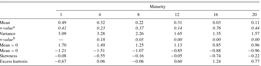
Table 1 sets out some summary statistics describing the
revisions history of published data of differing maturities— evaluating revisions over a 20-quarter window. Table2reports estimated heteroscedasticity, bias, serial correlation, and corre-lation parameters.
The summary statistics suggest that, on average, upward re-visions have been larger magnitude than downward rere-visions. However, the null hypothesis that mean revisions are zero can-not be rejected at the 5% level for any maturity. The variance of revisions is 3.09 percentage points for estimates with a ma-turity of one quarter. That is similar to the variance of whole-economy investment growth (3.12 percentage points). For re-cently released data there is little evidence of heteroscedasticity, but the variance of revisions does decline quite markedly once data have reached a maturity of 8 quarters. The null hypothesis that the variance of revisions is equal to that at maturity 1 is rejected at the 5% level for maturities beyond 8 quarters.
The bias was not found to be significant and hence was ex-cluded from the model. This is not surprising given that Table1 shows bias to be insignificant at all maturities. The measure-ment error variance parameters also map fairly easily from the summary statistics. The variance decay parameter suggests a
Table 2. Quarterly growth of whole economy investment—estimated parameters
half-life for measurement errors of 12 quarters. There is sig-nificant first-order negative serial correlation across revisions: successive quarters of upward/downward revision are therefore unusual. Revisions appear to have been negatively correlated with mature estimates, although the parameter is only signifi-cant at the 10% level.
Table 3 reports the parameters estimates from the Kalman
filter, while Table4sets out some standard diagnostic tests of the various residuals to give an indication of the degree to which modeling assumptions are violated in the dataset. Higher orders ofqwere not found to be statistically significant, therefore the transition equation does not include an autoregressive compo-nent.
Both the prediction errors for the published data and the smoothed estimates of the errors on the transition equations pass standard tests for stationarity, homoscedasticity, and ab-sence of serial correlation at the 5% level. Prediction errors are the “surprise” in the observable variables (i.e., official published data and alternative indicators) given the information available about previous time periods. These errors enter into the predic-tion error decomposipredic-tion of the likelihood funcpredic-tion. Standard maximum likelihood estimation therefore assumes that these errors are zero-mean, independent through time, and normally distributed. If this is not the case, then the Kalman filter does not provide an optimal estimator of the unobserved states. The er-rors surrounding predictions for the indicator variable are less well behaved. In particular, there is evidence of significant ser-ial correlation in these residuals. We have assumed that residu-als associated with the indicator variables are iid. This assump-tion could be relaxed in future work.
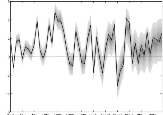
We next turn to the estimate of quarterly growth of whole economy investment—that is, the smoothed backcast. Figure1 reports the estimates of quarterly growth of whole economy in-vestment. Following the presentational convention of the GDP
Table 1. Quarterly growth of whole economy investment—revisions summary statistics, 1993Q1 to 2006Q4
Maturity
ap-value of a test that mean revision are zero at each maturity.
bp-value of a test that revisions variance at each maturity is smaller than revisions variance at maturity one.
178 Journal of Business & Economic Statistics, April 2012
Table 3. Estimated Kalman filter parameters
Parameter Standard error
True data parameters
Constant μ 1.121 0.238
Error variance σǫ2 3.217 0.673
Indicator parameters
Constant cs 1.177 0.219
Slope Zs 0.369 0.138
Error variance σv2s 2.629 0.567
and inflation probability forecasts (more commonly known as fan charts) presented in the Bank of England’s Inflation Re-porteach band contains 10% of the distribution of possible out-comes. In this application, because the normality assumption is not rejected by the data, the outer (90%) band is equivalent to a ±1.6 standard error bound.
The central point of the fan chart tracks the statistical agency’s published estimates quite closely once those estimates are mature. This follows from the fact that the heteroscedastic-ity and bias in measurement errors decline reasonably rapidly. Over the most recent past, the central point differs more materi-ally. This mainly reflects the higher measurement error variance attaching to earlier releases.
4.2 Real-Time Evaluation of the State Space Model
In this subsection we provide an evaluation of the real-time performance of the model. For this experiment, the evaluation period starts at s0=1998Q1 and terminates ats1=2002Q4. That is the model is estimated on samples from 1993Q1 to
1998Q1. The estimation period is then extended to include
observed data for the following time period, that is, 1998Q2. This is repeated until 2002Q4, which gives 20 evaluation ob-servations. For each run, we compare the performance of the smoothed backcast with that of the official published estimates available at the time the smoothed backcast was formed. Be-cause each official data release includes data points of differing maturities, we evaluate backcasting performance for each ma-turity from 1 to 24.
In standard forecasting applications, real-time performance is evaluated on the basis of forecast errors—often using the RMSE as a summary statistic. Evaluation of backcasts is more complex because we do not have observations of the “truth” as a
Figure 1. Fan chart for quarterly growth of investment and the of-ficial estimate (solid line). Each band contains 10% of the distribution of possible outcomes.
basis for evaluation. Instead, we evaluate performance of back-casting the profile of investment revealed 14 releases after the official data were published. That is, we compare the value of the smoothed backcast at timetof maturitynwith the data re-lease at timetof maturityn+14 to derive an RMSE-type metric ςn= s 1
1−s0+1
s1
t=s0(yˆt−y
t+n+14
t )2, whereyˆtis the smoothed
backcast ofyt made at maturityn in the case of the smoothed
data and is the published data otherwise.
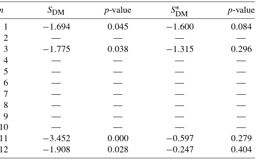
Figure2plotsςnfor published data and smoothed backcasts
for maturities 1 to 24. The backcasting errors appear smaller than the errors attaching to the official published estimates.
Table5 reports the results of Diebold–Mariano tests, SDM (Diebold and Mariano 1995) of the significance of the differ-ence in performance between backcasts and official published estimates for maturities 1 to 12.Harvey, Leybourne, and New-bold(1997) have proposed a small-sample correction for the above test statistic, SDM∗ . The table reports the test statistics for the null hypothesis that the two alternative backcasts are equally good. We also report probability values for these sta-tistics. Probability values below 0.05 indicate rejection of the null hypothesis in favor of the hypothesis that the state space model backcast is better than the early release in estimating the truth. Note that in a number of cases the Diebold–Mariano sta-tistics are reported as missing. This is because in these cases
Table 4. Model residual diagnostics
ˆ
ǫt vˆst εˆtT
ADF test: no constant or trend −6.114 −2.795 −5.405
ADF test: constant, but no trend −6.054 −2.781 −5.346
ADF test: constant and trend −5.984 −3.439 −5.401
Normality test 0.598 0.921 0.891
Serial correlation test: 1 lag 0.313 0 0.061
Serial correlation test: 4 lags 0.538 0 0.294
ARCH test: 1 lag 0.069 0.006 0.166
ARCH test: 4 lags 0.401 0.064 0.646
NOTE: Table reportsp-values for all tests except for the ADF tests, wheret-statistics is reported. Entries in bold indicate rejection of the null hypothesis at 5% significance level.
Figure 2. RMSE for maturities 1 to 24 for smoothed backcast (dashed line) and published data (solid line).
the estimated variance of the numerator of the statistic is neg-ative as is possible in small samples. For more details on this issue, see p. 254 inDiebold and Mariano(1995). The results show that the Diebold–Mariano test rejects the null hypothesis of equal forecasting ability in all available cases. On the other hand the modified test never rejects. We choose to place more weight on the results of the original, and more widely used, Diebold–Mariano test and conclude that there is some evidence to suggest that the state space model backcast is superior to the early release in estimating the truth.
5. CONCLUSIONS
We have articulated a state space representation of the signal extraction problem faced when using uncertain data to form a conjunctural assessment of economic activity. The model draws on the revisions history to proxy the uncertainty surrounding the latest published estimates. Therefore it establishes the ex-tent to which prior views on economic activity should evolve in light of new data and any other available measures, such as business surveys. The model produces estimates of the “true” value of the variable of interest, a backcast, that can be used as a cross-check of the latest published official data, or even to substitute for those data in any economic applications. Since
Table 5. Diebold–Mariano test results for maturities 1 to 12
n SDM p-value S∗DM p-value
we assume that official estimates asymptote to the truth as they become more mature, our backcasts amount to a prediction of the cumulative impact of revisions to official estimates.
In using backcasts to predict the cumulative impact of re-visions, one should, however, be alert to a number of caveats. First, we assume that the revisions history provides a good in-dication of past uncertainties. This assumption is likely to be violated where statistical agencies do not revise back data in light of new information or changes in methodology—in other words, the model is only applicable where statistical agencies choose to apply a rich revisions process. Second, we assume that the structures of both the data generating process (the tran-sition law) and the data production process (measurement equa-tions) are stable. Finally, the model is founded on a number of simplifying assumptions. In particular, the model is linear and stationary and the driving matrices are diagonal so that we can neither exploit any behavioral relationship between the variables of interest nor any correlation in measurement errors across variables.
ACKNOWLEDGEMENT
This paper represents the views and analysis of the authors and should not be thought to represent those of the Bank of England, Monetary Policy Committee, or any other organiza-tion to which the authors are affiliated. We would like to thank the Editor, the Associate editor, and an anonymous referee for extremely helpful comments on earlier versions of the paper. We have further benefited from helpful comments from Andrew Blake, Spencer Dale, Kevin Lee, Lavan Mahadeva, Tony Yates, and Shaun Vahey. We would also like to thank Simon Van Nor-den for his constructive and incisive comments especially on the relation between our model and comparable recent models in the literature.
[Received June 2008. Revised March 2009.]
REFERENCES
Akritidis, L. (2003), “Revisions to Quarterly GDP Growth and Expenditure Components,”Economic Trends, 601, 69–85. [174]
Ashley, J., Driver, R., Hayes, S., and Jeffery, C. (2005), “Dealing With Data Uncertainty,”Bank of England Quarterly Bulletin, 45 (1), 23–30. [174] Cameron, A. C., and Trivedi, P. K. (2005),Microeconometrics: Methods and
Applications, New York: Cambridge University Press. [175]
Castle, J., and Ellis, C. (2002), “Building a Real-Time Database for GDP(E),”
Bank of England Quarterly Bulletin, 42 (1), 42–48. [177]
Cunningham, A., Eklund, J., Jeffery, C., Kapetanios, G., and Labhard, V. (2009), “A State Space Approach to Extracting the Signal From Uncertain Data,” Working Paper 637, Queen Mary University of London. [175,176] Diebold, F. X., and Mariano, R. S. (1995), “Comparing Predictive Accuracy,”
Journal of Business & Economic Statistics, 13, 253–263. [178,179] Donald, S. G., and Newey, W. K. (2001), “Choosing the Number of
Instru-ments,”Econometrica, 69, 1161–1191. [175]
Garratt, A., and Vahey, S. P. (2006), “UK Real-Time Macro Data Characteris-tics,”The Economic Journal, 116 (509), F119–F135. [174,177]
Garratt, A., Lee, K., Mise, E., and Shields, K. (2008), “Real-Time Representa-tions of the Output Gap,”The Review of Economics and Statistics, 90 (4), 792–804. [174,175]
Harvey, A. (1989),Forecasting, Structural Time Series Models and the Kalman Filter, Cambridge: Cambridge University Press. [175]
Harvey, D. I., Leybourne, S. J., and Newbold, P. (1997), “Testing the Equality of Prediction Mean Square Errors,”International Journal of Forecasting, 13, 273–281. [178]
180 Journal of Business & Economic Statistics, April 2012
Howrey, E. P. (1978), “The Use of Preliminary Data in Econometric Forecast-ing,”Review of Economics and Statistics, 60 (2), 193–200. [173]
(1984), “Data Revision, Reconstruction, and Prediction: An Applica-tion to Inventory Investment,”The Review of Economics and Statistics, 66 (3), 386–393. [174]
Jacobs, J. P. A. M., and Van Norden, S. (2007), “Modeling Data Revisions: Measurement Error and Dynamics of “True” Values,” Les Cahiers de CREF 07-09, HEC Montréal. [174]
Kapetanios, G., and Yates, T. (2009), “Estimating Time-Variation in Measure-ment Error From Data Revisions; an Application to Forecasting in Dynamic Models,”Journal of Applied Econometrics, to appear. [174,175]
Mitchell, J. (2004), “Review of Revisions to Economic Statistics: A Report to the Statistics Commission,” Report No. 17, 2, Statistics Commission. [173] Öller, L.-E., and Hansson, K.-G. (2002), “Revisions of Swedish National Ac-counts 1980–1998 and an International Comparison,” discussion paper, Sta-tistics Sweden. [173]