Full Terms & Conditions of access and use can be found at
http://www.tandfonline.com/action/journalInformation?journalCode=ubes20
Download by: [Universitas Maritim Raja Ali Haji] Date: 12 January 2016, At: 00:29
Journal of Business & Economic Statistics
ISSN: 0735-0015 (Print) 1537-2707 (Online) Journal homepage: http://www.tandfonline.com/loi/ubes20
Derivative Pricing With Wishart Multivariate
Stochastic Volatility
Christian Gourieroux & Razvan Sufana
To cite this article: Christian Gourieroux & Razvan Sufana (2010) Derivative Pricing With Wishart Multivariate Stochastic Volatility, Journal of Business & Economic Statistics, 28:3, 438-451, DOI: 10.1198/jbes.2009.08105
To link to this article: http://dx.doi.org/10.1198/jbes.2009.08105
Published online: 01 Jan 2012.
Submit your article to this journal
Article views: 214
View related articles
Derivative Pricing With Wishart Multivariate
Stochastic Volatility
Christian G
OURIEROUXCREST, 92245 Malakoff Cedex, France, CEPREMAP, 75013 Paris, France, and Department of Economics, University of Toronto, Toronto, Ontario M5S 3G7, Canada (c.gourieroux@utoronto.ca)
Razvan S
UFANADepartment of Economics, York University, Toronto, Ontario M3J 1P3, Canada (rsufana@yorku.ca)
This paper deals with the pricing of derivatives written on several underlying assets or factors satisfying a multivariate model with Wishart stochastic volatility matrix. This multivariate stochastic volatility model leads to a closed-form solution for the conditional Laplace transform, and quasi-explicit solutions for derivative prices written on more than one asset or underlying factor. Two examples are presented: (i) a multiasset extension of the stochastic volatility model introduced by Heston (1993), and (ii) a model for credit risk analysis that extends the model of Merton (1974) to a framework with stochastic firm liability, stochastic volatility, and several firms. A bivariate version of the stochastic volatility model is estimated using stock prices and moment conditions derived from the joint unconditional Laplace transform of the stock returns.
KEY WORDS: Credit default swap; Credit risk; Derivative pricing; Stochastic volatility; Wishart pro-cess.
1. INTRODUCTION
The standard Black–Scholes model (Black and Scholes 1973) is not flexible enough to reproduce some stylized facts observed on derivative prices such as the smile effect, that is a U-shaped relationship between the implied Black–Scholes volatility and the strike price (for any given residual maturity). It is well known that a smile can be created by introducing sto-chastic volatility in the Black–Scholes model. This approach was introduced by Hull and White (1987) and improved by Heston (1993), and Ball and Roma (1994), who changed the volatility dynamics to ensure a positive volatility.
Another stylized fact widely documented in the empirical lit-erature and not captured in the Black–Scholes framework is the skewness of the univariate implied volatilities as a function of the stock price, called the leverage effect. The leverage effect can be recovered at least in two different ways:
(i) It can be created by considering a stochastic volatility model with an instantaneous correlation between the stock re-turn and volatility shock (see, e.g., Heston 1993). In this ex-tension the instantaneous correlation is conditional on a rather small information set including the past values of the asset re-turn and volatility shock only.
(ii) An alternative way for creating a leverage effect consists in increasing the information set. The conditional correlation depends on the selected information set, and the asset return and stochastic volatility can be conditionally uncorrelated for a large information set and conditionally correlated for a smaller information set as a consequence of the covariance analysis equation. More precisely, let us consider two information sets at timet:ItandJt, withIt⊂Jt. The covariance analysis equation written for the change in returnrand volatilityσ is
Cov(drt,dσt|It)
=Cov[E(drt|Jt),E(dσt|Jt)|It] +E[Cov(drt,dσt|Jt)|It].
Thus, we can have simultaneously Cov(drt,dσt|Jt)=0 and Cov(drt,dσt|It)=0. This case arises when a common unob-servable factor is introduced in the drifts ofdrtanddσt[i.e., in E(drt|Jt)andE(dσt|Jt)] and then integrated out. Loosely speak-ing, a leverage effect observed on a single asset can be recov-ered by considering an appropriate multifactor framework and integrating out the effect of some of the factors.
The present paper introduces a multivariate model in which the stochastic volatility matrix follows the Wishart autoregres-sive (WAR) process introduced by Bru (1991) and studied in Gourieroux, Jasiak, and Sufana (2009) (see also Gourieroux 2006for a survey). The Wishart process is a multivariate exten-sion of the CIR process (Cox, Ingersoll, and Ross1985), and allows us to jointly model not only the dynamics of volatilities, but also the evolution of covolatilities. The WAR specification ensures by construction the positive definiteness of the stochas-tic volatility matrix.
An advantage of the multivariate stochastic volatility model presented in this paper is the closed-form expression of the conditional Laplace transform (moment generating function). Since the conditional Laplace transform is the basis for pric-ing derivatives (Duffie, Pan, and Spric-ingleton2000), the model implies quasi-explicit solutions for derivative prices. The mul-tivariate stochastic volatility model for asset returns provides a more accurate analysis of the joint risks captured in the co-volatilities, a focus on the risk premia corresponding to these covolatilities, and is needed for pricing derivatives written on several underlying assets or factors. The multivariate stochas-tic volatility model can also be applied with some unobservable
© 2010American Statistical Association Journal of Business & Economic Statistics
July 2010, Vol. 28, No. 3 DOI:10.1198/jbes.2009.08105
438
factors in order to capture the observed leverage effect in the al-ternative way mentioned above, or to model default dependence and price basket derivatives in credit risk. The introduction of unobservable common factors is required by the Basel 2 regula-tion concerning internal risk models (Basel Committee on Bank Supervision2001). The cost of using the multivariate model is the large number of parameters, which increases the complex-ity of the model and represents the usual curse of dimension-ality encountered in multivariate stochastic volatility models. It can be solved by considering WAR factor models or by in-troducing appropriate parameter restrictions (Bonato, Caporin, and Ranaldo2008; Gourieroux, Jasiak, and Sufana2009).
Two examples of multivariate stochastic volatility models illustrate the flexibility and tractability of the general frame-work. The first model is a multiasset extension of the stochastic volatility model introduced by Heston (1993), that specifies a price equation with a volatility-in-mean effect to capture the risk premia on each asset. By introducing interactions between covolatilities and expected returns, it will also capture the ten-dency for the volatility and stock price to move together (i.e., the leverage effect) without assuming an instantaneous corre-lation between the stock return and the volatility-covolatility innovations. The second example of the general multivariate model is a model for credit risk analysis that extends the model of Merton (1974) to a framework with stochastic firm liabil-ity, stochastic volatilliabil-ity, and more than one firm. The extended model allows for default dependence and a joint pricing of risky bonds and credit default swaps.
The paper is organized as follows. Section2introduces the factor model with multivariate stochastic volatility. Then we de-rive a closed-form solution for the conditional Laplace trans-form of the joint process of integrated factors, volatilities, and covolatilities. This derivation requires the analysis of the Ric-cati differential system associated with the WAR process. We prove that the structure of the Riccati equations allows for an explicit solution of this differential system. Section 3 studies two examples of multivariate stochastic volatility models, a multiasset model and a credit risk model, and explains how to obtain solutions for derivative prices. In Section4, a bivariate version of the model is estimated by the generalized method of moments, using daily stock prices and moment conditions derived from the joint unconditional Laplace transform of the stock returns, and illustrates the differences relative to tradi-tional multivariate models. Section 5 concludes. Proofs and other technical results are gathered in appendices.
2. FACTOR MODEL WITH MULTIVARIATE
STOCHASTIC VOLATILITY
In this section we introduce and discuss a model for the joint evolution of a vector of stochastic factors, and of their associ-ated stochastic volatility matrix.
2.1 The Factor Model
Let us considernpositive stochastic factors whose values at timetare represented in ann-dimensional vectoryt. The(n,n)
infinitesimal stochastic volatility matrix of the factors is de-noted by t. The joint dynamics of logyt andt is given by the stochastic differential system:
dlogyt=μ+(Tr(D1t), . . . ,Tr(Dnt))′dt
+t1/2dWtS, (1)
dt=(KQ′Q+Mt+tM′)dt+1t/2dWtσ(Q ′Q)1/2
+(Q′Q)1/2(dWtσ)′1t/2, (2)
where WtS and Wtσ are a n-dimensional vector and a (n,n) matrix, respectively, whose elements are independent unidi-mensional standard Brownian motions, μ is a constant n -dimensional vector,K is a scalar such thatK>n−1, andDi, i=1, . . . ,n,M,Qare(n,n)matrices withQ′Qinvertible. Tr denotes the trace operator and1t/2is the positive symmetric square root of the volatility matrixt.
The dynamics of the volatility matrix t in Equation (2) represents a continuous-time process of stochastic, symmet-ric, positive definite matrices. It corresponds to the continuous-time WAR introduced by Bru (1991) and studied in Gourieroux, Jasiak, and Sufana (2009) and Gourieroux (2006) as a tool for modeling the dynamics of volatility matrices. By construction, the Wishart specification of the volatility matrix ensures that, at any point in time, the factor volatilities and covolatilities sat-isfy the constraints imposed by the positive definiteness of the volatility matrix (see SectionA.1). An alternative specification of the volatility matrix assumes that the inverse oft follows a Wishart process. This extends the inverted gamma distribu-tion assumed in one-dimensional stochastic volatility models to get a closed form expression for the return density and to study its tail magnitude (see, e.g., Praetz1972; Clark1973; Blattberg and Gonedes 1974). The direct Wishart specification used in our framework is more appropriate for deriving closed form ex-pressions for the moment generating functions and for pricing derivatives.
The drift in Equation (1) is an affine function of factor volatil-ities and covolatilvolatil-ities:
Et(dlogyi,t)= [μi+Tr(Dit)]dt, i=1, . . . ,n, (3)
whereEtdenotes the expectation conditional on the information available at timet. Without loss of generality we can restrictDi to be symmetric, since Tr(Dit)=Tr(12(Di+D′i)t).
Even for a rather small dimension n, the model involves a large number of parameters equal ton2(n+5)/2+n+1. For instance, there are 40 and 77 parameters for n=3 andn=4, respectively. This is the curse of dimensionality encountered in multivariate volatility models. It explains the flexibility of the model, but can create difficulties for estimation. A reduction in the number of parameters can be achieved by considering WAR-in-mean models with factors as discussed in Gourieroux, Jasiak, and Sufana (2009), or by introducing appropriate re-strictions on the parameters as in Bonato, Caporin, and Ranaldo (2008).
2.2 Affine Property and Conditional Laplace Transform
The joint process(logyt, t)is an affine process, that admits drift and volatility functions which are affine functions of logyt and t (see Duffie and Kan 1996 and Duffie, Filipovic, and Schachermayer2003for the definitions and analysis of standard affine processes). The results in SectionA.2show that the affine property is satisfied for the drift and volatility of(logyt, t).
The general theory of affine processes implies that the con-ditional Laplace transform (moment generating function) of the joint process(logyt, t)is exponential affine. The conditional Laplace transform of the joint process(logyt, t)and of its in-tegrated values is defined by
t,h(γ , γ0,γ ,C,c0,C) C,C can be real or complex whenever the expectation exists. The property below is a direct consequence of general results on affine processes (see Duffie, Filipovic, and Schachermayer 2003).
Proposition 1. The conditional Laplace transform of the affine process (1)–(2) is
t,h(γ , γ0,γ ,C,c0,C)
=expa(h)′logyt+Tr(B(h)t)+b(h)
, (5)
wherea,b, and the symmetric matrixB satisfy the system of Riccati equations: Proof. SeeAppendix B.
The differential system (6)–(8) involves parameters γ , γ0, C,c0,whereasγ ,Cdefine the initial conditions. The differen-tial equation foraadmits the explicit solution
a(h)=γh+γ .
Then, system (6)–(8) can be solved recursively. The Riccati Equation (7) provides the matrix B(h)and finally the form of b(h)is obtained substitutinga(h)andB(h)by their expressions in Equation (8).
In general, Riccati equations do not admit closed-form so-lutions and have to be solved numerically. The main result of the paper is the following proposition which provides a closed-form solution for Riccati Equation (7) in some special cases.
This is an example of multidimensional Riccati equation with a fundamental system of solutions (see Walcher1986,1991for a general definition, and Grasselli and Tebaldi2008for a dis-cussion of quadratic models, which do not include the present WAR process).
Proposition 2. Let us assumeγ=0, and the existence of a symmetric matrixB∗which satisfies
M′B∗+B∗M+2B∗Q′QB∗+1
The solutionB(h)is given by
B(h)=B∗+exp[(M+2Q′QB∗)h]′
The expression of b(h) can be derived by integrating Equa-tion (8):
Proof. SeeAppendix D.
The expression of B(h) in Proposition 2 admits a closed form. Indeed, up to an appropriate change of basis, the matrix exp[(M+2Q′QB∗)u]can be written under a diagonal or trian-gular form, whose elements are simple functions ofu (exponen-tial or exponen(exponen-tial times polynomial), which can be explicitly integrated between 0 andh.
The existence of a symmetric solutionB∗ of the quadratic system (9) in Proposition2implies joint restrictions on the pa-rameters and on the argument of the conditional Laplace trans-form.
Proposition 3. Under the conditions of Proposition2, ifγ,C are real, there exists an orthonormal basisei,i=1, . . . ,n,such
Proof. SeeAppendix E.
The restriction in Proposition3is related to the existence of the real conditional Laplace transformst,h in Equation (4). Since the stochastic volatility matrix is positive definite, the function exptt+hTr(Cu)duis integrable for any negative def-inite matrixC. However, the presence of stochastic volatility will increase the tails of the factor return distribution and there-fore the argumentγcannot be too large.
Under additional conditions on the parameters, we can de-rive explicit expressions for the solutionB∗ of the system (9), and for the coefficientsB(h)andb(h)in the conditional Laplace transform (5) without considering a diagonal or triangular de-composition of exp[(M+2Q′QB∗)u].
Proposition 4. LetŴ=12γγ′+ni=1γiDi+C, and assume that:
(i) (Q′Q)−1Mis a symmetric matrix, (ii) M′(2Q′Q)−1M−Ŵis positive definite.
Then, we get
B∗= −(2Q′Q)−1M
+(2Q′Q)−1/2(2Q′Q)1/2(M′(2Q′Q)−1M−Ŵ)
×(2Q′Q)1/21/2(2Q′Q)−1/2. (12)
Proof. SeeAppendix F.
In particular, we get the following corollary, by noting that (Q′Q)−1M=(Q′Q)−1/2M(Q′Q)−1/2 is symmetric whenM is symmetric andMand(Q′Q)1/2commute.
Corollary 5. LetP=(2Q′Q)1/2,Ŵ=21γγ′+ni=1γiDi+ C, and assume that:
(i) M′=M, (ii) PM=MP,
(iii) M2−PŴPis positive definite.
Then, denotingG= −(M2−PŴP)1/2, the matrixB∗is given by
B∗=P−1[G−M]P−1, (13)
and the expressions ofB(h)andb(h)are
B(h)=P−1
G−M+exp(Gh)
(PCP−G+M)−1
+1
2(Id−exp(2Gh))G −1
−1
exp(Gh)
P−1, (14)
b(h)=
γ′μ+γ0+c0+ K
2 Tr(G−M)
h
−K 2 log det
Id+1
2(PCP−G+M)
×(Id−exp(2Gh))G−1
. (15)
Proof. SeeAppendix G.
When the parameters do not satisfy the restrictions of Propo-sition4, the solutionB∗of Equation (9) has to be found numer-ically or the Riccati Equation (7) can be solved by applying the linearization technique considered in Fonseca, Grasselli, and Tebaldi (2005) (see also Buraschi, Cieslak, and Trojani 2007, appendix A.5).
3. MULTIVARIATE EXTENSIONS OF HESTON
AND MERTON MODELS
In this section we present two illustrations of models with multivariate stochastic volatility. The first illustration is an ex-tension to the multiasset framework of the stochastic volatility model introduced by Heston (1993). The second illustration is a model for credit risk analysis.
3.1 A Stochastic Volatility Model for Asset Prices
3.1.1 The Model. Let us consider a market with one risk-free asset andnrisky assets. The risk-free rateris assumed to be constant, whereas the infinitesimal geometric returns of the risky assets are represented in an-dimensional vectordlogst, withstbeing the vector of asset prices at timet. The (infinites-imal) stochastic volatility matrix of the risky returns is denoted byt.
The model for thenrisky assets is obtained from the multi-variate stochastic volatility model in Section2by replacingyt withst. Thus, the joint dynamics of logstandtis given by the stochastic differential system:
dlogst=
μ+(Tr(D1t), . . . ,Tr(Dnt))′
dt
+t1/2dWtS, (16)
dt=(KQ′Q+Mt+tM′)dt+t1/2dWtσ(Q′Q)1/2
+(Q′Q)1/2(dWtσ)′t1/2, (17)
where the notation is explained in Section2.
The volatility matrix in the drift of the price Equation (16) accounts for a risk premium. Section A.3 proves that, if the matrixDi is symmetric positive semidefinite for anyi, the risk premium is positive: Tr(Di)≥0, and that the risk premium is an increasing function of risk: Tr(Di)≥Tr(Di∗), for any ≫∗, and for anyi, where≫denotes the standard order-ing on symmetric matrices. Moreover, despite the assumption of independence betweenWtSandWtσ, this multivariate model is able to capture the leverage effect observed separately on a single asset. The reason is that by introducing for instance the covolatility between assets 1 and 2 in the expressions of the ex-pected return and volatility of asset 1, we can introduce a ten-dency for the volatility and return of asset 1 to move together when this unobserved stochastic covolatility is integrated out. This argument is valid for any number of additional assets in-troduced in the system. By increasing their number, we get a larger number of unobserved covolatility factors.
As a consequence of Propositions1and2, a closed-form so-lution can be derived for the conditional Laplace transform of the log asset pricesEt[exp(γ′logst+h)], which fully character-izes the conditional distribution of the asset returns:
Et[exp(γ′logst+h)] =t,h(0,0,γ ,0,0,0).
As usual, the introduction of stochastic volatility increases the tail magnitude of the stock returns. In the present framework, it is easily checked that the Laplace transform admits a series expansion in a neighborhood of zero and the power moments of stock returns exist at any nonnegative order. Thus, the tail increase due to Wishart stochastic volatility does not imply the nonexistence of some moments of stock returns.
The associated transition of the stock returns can be derived by inverting the Fourier transform, which is the Laplace trans-form evaluated at pure imaginary arguments, or in a more direct way. Indeed, for a given volatility path, the return process is multivariate Gaussian. The conditional distribution of logst+h
given(logst,t)is normal with mean
and variance–covariance matrix tt+hudu. Thus the transi-tion of logst+h given (logst, t) is deduced by integrating out the cumulated volatilitytt+hudugivent. The distrib-ution of the integrated volatilitytt+huduis characterized by Et[exp
Thus, the volatility process is a CIR process and the model re-duces to the specification introduced by Heston (1993). In this case, the conditional Laplace transform of the log asset prices is
Thus, the multiasset model in Equations (16) and (17) can be regarded as a multivariate extension of Heston’s model.
3.1.2 Derivative Pricing. The closed-form expression of the conditional Laplace transform given in Proposition 2 can be used to price derivatives written on the underlying assets by using the transform analysis (Duffie, Pan, and Singleton 2000). It allows us to avoid numerical approximations based on multibranches trees introduced in the multiasset framework (see, e.g., Boyle 1988; Boyle, Evnine, and Gibbs 1989; Ho, Stapleton, and Subrahmanyam1995; Chen, Chung, and Yang 2002), or expansions around the constant volatility hypothesis (see, e.g., Hull and White1987). Without loss of generality, we can assume a zero risk-free rate.
For derivative pricing, we need to discuss the form of the joint process(logst, t)under the risk-neutral distribution, and the link between the historical and risk-neutral parameters. Un-der differentiability conditions on Un-derivative prices, it is known
from Girsanov theorem that the change of density for period (t,t+h)between the historical and risk-neutral distributions is of the type change of probabilities and thus the coefficients in the stochas-tic discount factor are constrained by both the unit mass restric-tion and the martingale condirestric-tion on stock prices.
Proposition 6. Under the risk-neutral distribution, the joint process (logst, t) satisfies a stochastic differential system with volatility equal to the historical volatility and a modified drift:
whereE∗t denotes the conditional expectation under the risk-neutral probability, andeiis the canonical vector with zero com-ponents except for theith component which is equal to 1.
Proof. SeeAppendix C.
The risk premium on the Brownian motion of the return equation is fixed by the martingale condition (seeAppendix C), whereas the risk premia corresponding to the volatilities– covolatilities (that areCt) can be fixed arbitrarily as a conse-quence of market incompleteness (see, e.g., Garman1977).
The stochastic system under the risk-neutral probability has the same form as the stochastic system under the historical probability if the volatility risk premiaCt=C∗ are constant. Indeed, the former differential system corresponds to
Et∗(dlogst)= intercept in the volatility drift stays the same, whereas the ma-trix of “mean-reverting parameters” can be fixed arbitrarily.
The risk-neutral conditional Laplace transform t∗,h(γ , γ0,
γ ,C,c0,C)is defined as in Equation (4), withEt replaced by E∗
t. IfCt=C∗, it can be computed in closed form under the pa-rameter restrictions in Proposition2, after replacing the histori-cal parameters by the risk-neutral ones. As explained in Duffie, Pan, and Singleton (2000), the risk-neutral conditional Laplace transform is the basis for derivative pricing since it can be used to obtain explicit or quasi-explicit prices for various derivatives. For example, t∗,h(0,0,γ ,0,0,0) is the price at time t of a European derivative with exponential payoff exp[γ′logst+h]at
timet+h. European options and other derivatives with more complex payoffs are priced using Fourier inversion techniques, where the Fourier transform is simply the Laplace transform evaluated at pure imaginary arguments.
3.2 Credit Risk Model
The multivariate stochastic volatility model can also be ap-plied to credit risk analysis by considering the asset values and liabilities of the firms as the basic contingent claims. It defines a multifactor model for a simultaneous pricing of risky bonds and credit default swaps.
In the standard framework of the firm value model introduced by Merton (1974), the potential time to defaulth, say, is prede-termined, and the values of the stock, bonds, and credit default swaps corresponding to a given firmiare defined from the con-ditional risk-neutral distribution of its assetAi,t+hand liability Li,t+h at datet+h. More precisely, assuming a zero risk-free rate, the value at datet of a zero-coupon bond with residual maturityhissued by the firmiis
Bi(t,t+h)=E∗t
whereE∗t denotes the conditional expectation with respect to the risk-neutral probability and the first component takes into account the recovery rate when default occurs. The value at date tof the equity is
Si,t=Et∗[(Ai,t+h−Li,t+h)+],
whereas the value of the credit default swap with residual ma-turityhis
In the basic Merton’s model, the debt amountLi,t+his assumed predetermined, and the asset value follows the one-dimensional Black–Scholes model (the same assumption is made in the practical approach developed by Moody’s KMV for credit risk; see, e.g., Crosbie and Bohn2003). As a consequence, we get a one-factor model, where all derivative prices are deterministic functions of the asset value at datetonly.
However, the corporate liability is clearly as varying as the asset value when taking new credits is easy, or when these credit lines are not completely used, and often both underlying vari-ables increase together when the firm comes closer to default. Note that the existing credit lines can still be used even after default (see Gourieroux and Tiomo2007). An extension to the framework of stochastic liability has been performed by Sta-pleton and Subrahmanyam (1984) with a multivariate Black– Scholes model. The results of Section2allow for the extension to stochastic volatility and multifirm framework.
3.2.1 Extension to Stochastic Volatility. Let us first con-sider a given firm. We can represent the joint dynamics of the asset value and liability by
cluded in the drift do not admit an interpretation as risk pre-mia since the firm’s asset and liability values are not directly traded on a market. Their interpretation in this context is the following. Let us for a while consider Merton’s model with a constant debt level, but stochastic volatility. Default may occur for at least two reasons:
(i) the asset value has a decresing trend and reaches the lia-bility level, or
(ii) the asset value has a constant mean, but a large volatility increase causes the asset value to cross the liability level.
In the first case, the decreasing trend may be due to a prob-lem with an economic fundamental of the firm, whereas in the second case the fundamental may be stable, but the asset value will be below the debt level during a transitory period only. In the latter situation, the medium-term rating of the firm allows it to increase its debt in order to stimulate its investments, and as a result increase the asset value. This explains why correlated evolutions of the asset and liability values are observed when the risk increases, and this effect is captured by the two drift terms.
3.2.2 Extension to Several Firms. The model is easily ex-tended to several firms, in order to distinguish the firm idio-syncratic effects from the common effects. This distinction is crucial in the analysis of large portfolios of bonds or credit de-fault swaps. Indeed, the idiosyncratic risks can be diversified by increasing the size of the portfolio. But the common effect still remains for large portfolios. The introduction of such a com-mon factor is required in the approach of Basel 2 regulation to capture the default dependence (Basel Committee on Bank Supervision2001).
Let us consider for the exposition a homogeneous portfolio where the n firms are considered equivalent. The model be-comes
where the common risk factor satisfies
dt=(KCQC′QC+MCt+tMC′)dt
+t1/2dWtσ(QC′QC)1/2+(QC′QC)1/2(dWtσ)′1t/2,
and the idiosyncratic risk factors are such that
di,t=(KIQI′QI+MIi,t+i,tMI′)dt
+i1,/t2dWiσ,t(QI′QI)1/2+(QI′QI)1/2(dWiσ,t)′i1,/t2.
As usual the idiosyncratic and common innovations WtS,WiS,t, i=1, . . . ,n,Wtσ,Wiσ,t,i=1, . . . ,n,are assumed independent. Whereas a large part of the literature on “correlated defaults” focuses on “reduced form models,” the framework above pro-vides a structural model easy to implement and sufficiently flex-ible to replicate the expected patterns of the term structure of default correlations.
4. EMPIRICAL APPLICATION
4.1 The Moment Method
Various methods are available in the literature for estimating stochastic volatility models. In our framework it is convenient to exploit the closed-form expression of the conditional Laplace transform for the estimation of system (16)–(17). The uncondi-tional Laplace transform is used to derive exact uncondiuncondi-tional moments and cross-moments of asset returns, and then a gener-alized method of moments is applied.
Let us consider a model for two stock prices where
D1=
d
11 d13 d13 d12
, D2=
d
21 d23 d23 d22
,
Q′Q=(q2)Id, M=
m1 m3 m3 m2
.
Corollary 5 allows us to compute explicitly the uncondi-tional Laplace transforms of log stock returns Eexp(u′1rt+h), and Eexp(u′2rt+2h+u′1rt+h), where rt+h=logst+h−logst, and then derive exact moment expressions. The unconditional Laplace transformEexp(u′1rt+h)is derived as follows:
Eexp(u′1rt+h)=EEtexp(u′1rt+h)
=Et,h(0,0,u1,0,0,0)
=exp(b(h))EexpTr(B(h)t)
=exp(b(h))det(Id+q2M−1B(h))−K/2,
where the third equality uses the unconditional Laplace trans-form of a Wishart variable, and b(h)and B(h)are computed using Corollary 5 with γ =0, γ0=c0=0, C=C=0, and
γ=u1. The expression forEexp(u′2rt+2h+u′1rt+h)is obtained similarly. Ifu′1=(i,j)andu′2=(k,l), then
exp(u′2rt+2h+u′1rt+h)
=
s1,t+2h s1,t+h
k s2,t+2h
s2,t+h
l s1,t+h
s1,t
i s2,t+h
s2,t
j .
We consider 17 exact moment conditions with the following values of (u′2,u′1): (0, 0, 1, 0), (0, 0, 0, 1), (0, 0, 2, 0), (0, 0, 0, 2), (0, 0, 1, 1), (1, 0, 1, 0), (0, 1, 0, 1), (1, 0, 0, 1), (0, 1, 1, 0), (1, 0, 2, 0), (0, 1, 0, 2), (1, 0, 0, 2), (0, 1, 2, 0), (2, 0, 2, 0), (0, 2, 0, 2), (2, 0, 0, 2), (0, 2, 2, 0). The generalized method of mo-ments is applied with these 17 moment conditions to estimate the 13 parameters of the model. The weighting matrix is esti-mated according to Newey and West (1987), with a lag length of 20.
4.2 The Data
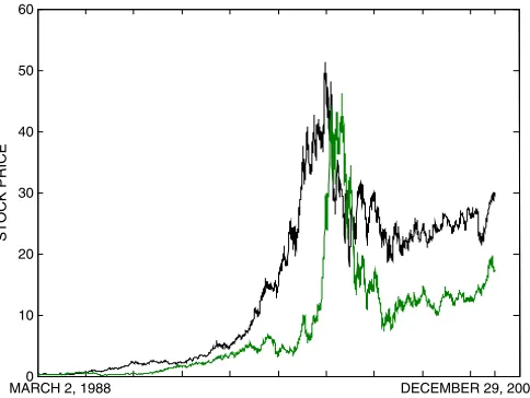
The estimation uses daily close prices adjusted for dividends and splits for Microsoft and Oracle stocks, which had the largest market capitalizations in the application software industry over the selected sample period. The data were obtained from the Yahoo website, for the period from March 2, 1988 to Decem-ber 29, 2006. The numDecem-ber of observations is 4,751. Table1 pro-vides summary statistics and shows that the Oracle return had a higher mean and was more volatile over the sample period,
Table 1. Summary statistics of the stock returns
Mean Std. deviation Skewness Kurtosis Minimum Maximum
0.0012 0.0224 0.0930 7.0946 −0.1560 0.1958
0.0016 0.0358 0.4638 13.634 −0.3175 0.4375
Lagi ρ1(i) ρ2(i) ρ12(i) ρ21(i)
0 0.4097
1 −0.0146 −0.0556 0.0028 −0.0342
2 −0.0255 −0.0528 −0.0255 −0.0441
3 −0.0349 −0.0222 −0.0252 −0.0071
4 −0.0216 −0.0064 −0.0063 0.0014
NOTE: The first row of statistics refers to the Microsoft stock return, the second refers to the Oracle stock return.ρ1(i)andρ2(i)are the autocorrelations at lagifor the Microsoft and Oracle stock returns,ρ12(i)andρ21(i)are the cross-correlations at lagibetween the Microsoft and Oracle stock returns, and between Oracle and Microsoft stock returns, ρ12(0)is the correlation of the two stock returns.
with a standard deviation about 60% larger than that of the Mi-crosoft return. Both returns exhibit skewness and kurtosis, with relatively higher values for Oracle. The contemporaneous cor-relation between the stock returns is 0.4097, but the (uncondi-tional) autocorrelations and cross-correlations at lags 1 to 4 are small. Figure1provides a plot of the two stock prices.
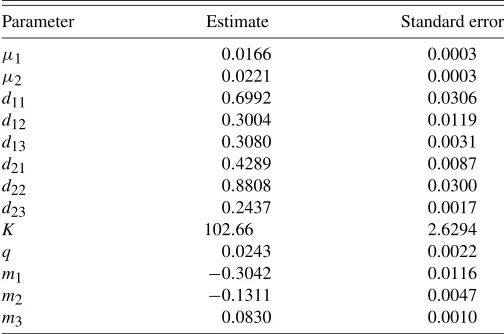
4.3 The Estimation Results
Table 2 reports the estimation results. All parameter esti-mates are significant at conventional levels. The estiesti-mates for the autoregressive matrixM indicate a mean-reverting behav-iour of the volatility matrix. In particular, the significance ofm3 reveals the importance of the covolatility (or, equivalently, of the correlation) of the stock prices in the dynamics of volatil-ities and prices. Let us discuss the estimates of the risk pre-mia parameters inD1andD2. Their estimated eigenvalues and eigenvectors are given in Table3. The risk premia matrices have full rank, and therefore cannot be represented by the single ef-fect of the volatility of a market portfolio. The risk premium on each stock depends on the volatilities of both assets, and also on their covolatility, with a relatively higher sensitivity to the volatility of the same stock.
Figure 1. Daily prices for the Microsoft stock (solid line) and Ora-cle stock (dotted line). A color version of this figure is available in the electronic version of this article.
Table 2. Estimation results of the bivariate model of stock returns
Parameter Estimate Standard error
μ1 0.0166 0.0003
μ2 0.0221 0.0003
d11 0.6992 0.0306
d12 0.3004 0.0119
d13 0.3080 0.0031
d21 0.4289 0.0087
d22 0.8808 0.0300
d23 0.2437 0.0017
K 102.66 2.6294
q 0.0243 0.0022
m1 −0.3042 0.0116
m2 −0.1311 0.0047
m3 0.0830 0.0010
NOTE: The estimation results are obtained by the generalized method of moments ap-plied to 17 moment conditions and 4,750 daily returns on Microsoft and Oracle stocks.
4.4 A Simulation Experiment
We further illustrate the estimation results by performing a simulation experiment. The system (16)–(17) is used to gener-ate sample paths, with the initial stock prices set to the values on the first day in the actual sample. The values of the parameters are fixed according to the estimated values in Tables2 and3, except for the eigenvalues of the risk premia parameters D1 andD2. Indeed the eigenvalues of the risk premia parameters are important for financial purposes, and also likely among the parameters more difficult to estimate. In Table3the estimated eigenvalues ofD1andD2are such that the first eigenvalue of D1is a proportionα1=0.1329 of the sum of both eigenvalues, while forD2the proportion of the sum represented by the first eigenvalue isα2=0.2462. In the experiment we consider the values 0.125 and 0.25 for each ofα1andα2. The eigenvectors and the remaining parameters are fixed at the values in Tables2 and3.
A simulated path is obtained using the exact discretization of the estimated continuous-time Wishart process for the volatility matrix, where the estimate ofKwas rounded to the nearest integer. As shown in Gourieroux, Jasiak, and Sufana (2009), when K is integer, the exact discretization of the process in Equation (17) is the discrete-time Wishart process:
t=
K
k=1 xktxkt′ ,
where
xk,t+h=Mdxkt+εk,t+h, εk,t+h∼N(0, d),
and
Md=exp(Mh), d=q2
h
0
exp(Mu)[exp(Mu)]′du,
Table 3. The estimated eigenvalues and eigenvectors ofD1andD2
D1 D2
Eigenvalues 0.1329 0.8668 0.3225 0.9872
Eigenvectors 0.4778 −0.8785 −0.9165 0.4001
−0.8785 −0.4778 0.4001 0.9165
and h is the time step. Under the conditions of Corollary 5, d can be computed explicitly asd=(1/2)q2[exp(2Mh)− Id]M−1.
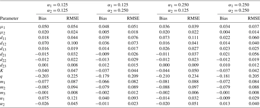
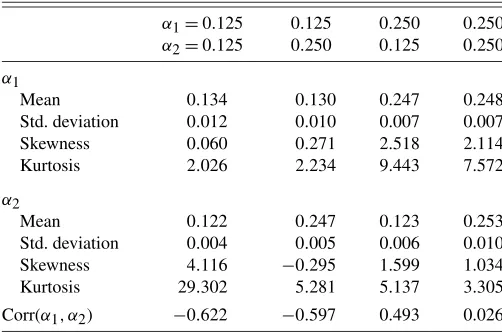
We consider two sample sizes for the simulated paths: 2520, representing 10 years of daily data, and 5,040, representing 20 years. The number of replications is 300. Tables 4 and5 display, for each parameter, the values of the mean bias and the root mean squared error divided by the absolute value of the initial parameter, for the 10 years and 20 years sample sizes, re-spectively. The values for the larger sample size in Table5are generally lower in absolute value than the corresponding val-ues in Table4. Both tables suggest thatqis the most difficult parameter to estimate, and is followed byα1in two of the four displayed cases, according to the root mean squared error val-ues. Table6reports summary statistics forα1andα2in the sim-ulation experiment. The relatively high kurtosis values suggest that the joint distribution ofα1andα2is non-Gaussian. The sign and magnitude of the correlation coefficient betweenα1andα2 varies significantly with their fixed values in the experiment.
5. CONCLUSION
The paper introduces a multivariate stochastic volatility model based on the Wishart autoregressive process that leads to closed-form solutions for the conditional Laplace transform, and quasi-explicit solutions for derivative prices written on more than one asset or underlying factor. In the Black–Scholes model with CIR stochastic volatility, a closed-form solution for option prices can be derived (Heston1993and Ball and Roma 1994). In this paper we have considered a multiasset exten-sion of this approach, where risk premia are introduced in the return equations and the CIR volatility process is replaced by a Wishart process for stochastic volatility matrices. The same approach is used to extend the standard Merton’s model for credit risk (Merton1974) by allowing for stochastic corporate liability, stochastic volatility, and more than one firm. These ex-tensions show that the Wishart process is a convenient tool for modeling the dynamics of volatility matrices.
The generalization to a multidimensional Wishart process provides flexibility and can help explain some stylized facts that a collection of independent univariate CIR processes can-not capture. This increased flexibility is both in the historical and risk-neutral frameworks. For instance, estimation of WAR processes from stock data showed that covariance terms are needed, and that the standard modeling based on independent CIR processes is rejected (see Gourieroux, Jasiak, and Sufana 2009). Similarly, in the risk-neutral world the WAR approach provides more realistic qualitative properties of the smile ef-fects, as seen in the analysis of skew, forward skew, and forward volatility performed by Fonseca, Grasselli, and Tebaldi (2005).
APPENDIX A: PROPERTIES OF THE VOLATILITY PROCESS
A.1 Positive Definiteness of the Wishart Process
Let us discuss the symmetry and positive definiteness of the Wishart process. The symmetry ofdt is immediately de-rived. Let us discuss the positive definiteness of dt. For this purpose, let us consider a quadratic form a′ta, where a is a n-dimensional vector. This quadratic form defines a
Table 4. Results of the simulation experiment for a sample size of 2520
α1=0.125 α1=0.125 α1=0.250 α1=0.250 α2=0.125 α2=0.250 α2=0.125 α2=0.250
Parameter Bias RMSE Bias RMSE Bias RMSE Bias RMSE
μ1 0.050 0.054 0.048 0.051 0.036 0.039 0.034 0.037
μ2 0.020 0.024 0.005 0.018 0.020 0.022 0.004 0.014
d11 0.018 0.044 0.039 0.076 0.073 0.111 0.022 0.060
d12 0.070 0.100 0.036 0.073 0.016 0.041 0.014 0.040
d13 0.016 0.019 0.014 0.017 0.026 0.027 0.023 0.025
d21 −0.015 0.032 −0.009 0.026 −0.011 0.037 0.021 0.056
d22 −0.012 0.022 −0.013 0.029 −0.012 0.023 −0.012 0.019
d23 0.001 0.008 0.012 0.015 0.000 0.009 0.010 0.012
K −0.040 0.047 −0.037 0.044 −0.044 0.050 −0.037 0.042
q −0.203 0.225 −0.179 0.209 −0.210 0.234 −0.181 0.205
m1 −0.077 0.087 −0.066 0.082 −0.081 0.088 −0.072 0.084
m2 −0.085 0.094 −0.079 0.089 −0.088 0.097 −0.079 0.088
m3 −0.001 0.008 −0.002 0.012 −0.002 0.006 −0.001 0.008
α1 0.075 0.121 0.040 0.093 −0.014 0.032 −0.009 0.029
α2 −0.026 0.045 −0.011 0.023 −0.020 0.051 0.013 0.040
NOTE: Bias and RMSE denote the mean bias and the root mean squared error divided by the absolute value of the initial parameter.
dimensional process with drift
Et[d(a′ta)] =(Ka′Q′Qa+a′Mta+a′tM′a)dt,
and volatility
Vt(a′dtb)=Vt[a′t1/2dWtσQb+a
′Q′(dWσ
t ) ′1/2
t b]
=Vt(a′t1/2dWtσQb+b′ 1/2
t dWtσQa)
=a′t1/2Vt(dWtσQb) 1/2 t a
+a′1t/2Covt(dWtσQb,dWtσQa) 1/2 t b
+b′1t/2Covt(dWtσQa,dWtσQb) 1/2 t a
+b′1t/2Vt(dWtσQa) 1/2 t b,
where Et and Vt denote the expected value and variance conditional on the information available at time t. Since Covt(dWtσa,dWtσb)=(a′b)Id dt, we obtain
Vt(a′dtb)
= [a′t1/2(b′Q′QbId)1t/2a+a′t1/2(b′Q′QaId)t1/2b
+b′t1/2(a′Q′QbId) 1/2 t a
+b′t1/2(a′Q′QaId)t1/2b]dt
=(a′tab′Q′Qb+2a′tbb′Q′Qa
+b′tba′Q′Qa)dt, (A.1)
Table 5. Results of the simulation experiment for a sample size of 5040
α1=0.125 α1=0.125 α1=0.250 α1=0.250 α2=0.125 α2=0.250 α2=0.125 α2=0.250
Parameter Bias RMSE Bias RMSE Bias RMSE Bias RMSE
μ1 0.035 0.040 0.037 0.044 0.026 0.032 0.025 0.031
μ2 0.016 0.022 0.009 0.018 0.016 0.022 0.010 0.021
d11 0.004 0.025 0.012 0.036 0.032 0.060 0.013 0.052
d12 0.025 0.050 0.033 0.065 0.010 0.036 0.008 0.043
d13 0.011 0.014 0.011 0.014 0.020 0.022 0.017 0.021
d21 −0.005 0.020 −0.003 0.028 −0.005 0.032 0.014 0.047
d22 −0.014 0.033 −0.007 0.026 −0.019 0.037 −0.011 0.031
d23 0.004 0.009 0.011 0.013 0.002 0.008 0.011 0.013
K −0.023 0.036 −0.027 0.040 −0.023 0.036 −0.028 0.040
q −0.092 0.124 −0.126 0.166 −0.107 0.143 −0.112 0.151
m1 −0.044 0.058 −0.053 0.067 −0.048 0.067 −0.051 0.064
m2 −0.051 0.063 −0.056 0.073 −0.060 0.072 −0.057 0.069
m3 −0.004 0.013 −0.002 0.011 −0.004 0.013 −0.003 0.011
α1 0.015 0.069 0.031 0.084 −0.010 0.029 −0.008 0.032
α2 −0.018 0.031 −0.007 0.022 −0.015 0.048 0.006 0.033
NOTE: Bias and RMSE denote the mean bias and the root mean squared error divided by the absolute value of the initial parameter.
Table 6. Summary statistics forα1andα2for a sample of size 2520
Let us now consider what arises whentreaches the bound-ary of the set of symmetric positive definite matrices. There exists a nonzero vector a in the kernel of t which satisfies a′ta=0, and alsota=0. In this case, we have
Vt[d(a′ta)] =0,
and
Et[d(a′ta)] =K(a′Q′Qa)dt>0,
wheneverQ′Qis invertible anda=0. Thus, we get a determin-istic reflection towards positivity when the boundary is reached.
A.2 Stochastic Properties of the Risk Premia
Similar computations provide the conditional covariance be-tween two quadratic forms based ondt:
Covt(a′dta,b′dtb)=4a′tba′Q′Qb dt, (A.3)
and
Covt(a′dta,b′dtc)
=2[a′tba′Q′Qc+a′tca′Q′Qb]dt. (A.4)
The result in (A.3) allows us to derive the volatility of Tr(D dt), where D is a symmetric positive definite matrix. SinceDcan be decomposed asD=ni=1aia′i, we get
The result above is modified ifDis not positive definite. The de-composition becomesD=ni=1εiaia′i, whereεi= ±1. A sim-ilar computation provides
Vt[Tr(D dt)] =4 Tr(D+tD+Q′Q)dt,
whereD+=ni=1aia′i is derived fromDby replacing all the eigenvalues by their absolute values. Similarly, using (A.4) we have
Note that all these second-order conditional moments are affine functions oft.
A.3 Positivity of the Risk Premia
We now prove that the risk premium is an increasing func-tion of risk, if the matrix D is symmetric positive semidefi-nite. A symmetric positive semidefinite matrixDcan be written asD=nj=1λjmjm′j, whereλjandmj are the eigenvalues and eigenvectors ofD, respectively. Thus, we get
Tr(D)=Tr
where the last equality and inequality follow since we can com-mute under the trace operator, λj>0, ∀j, and is positive definite. The risk premium is an increasing function of risk if and only if
Tr(D)≥Tr(D∗) for any≫∗,
or equivalently,
Tr(D(−∗))≥0 for any−∗≫0.
This condition is satisfied ifDis symmetric positive semidefi-nite.
APPENDIX B: CONDITIONAL LAPLACE TRANSFORM
The exponential affine expression of the conditional Laplace transform is a well-known property of affine processes (see, e.g., Duffie, Filipovic, and Schachermayer2003). Therefore, we only look for the generalized matrix Riccati equations satisfied by functionsa,B, andb. We have
Using the definitions of the affine processes in Equations (1), (2), and the result (A.5) derived inAppendix A, we have
the terms multiplying logyt,t and the intercept must be the same in the two expressions above. Identifying the correspond-ing terms and takcorrespond-ingdt→0, we derive the differential equa-tions
The initial conditions follow from
t,0=exp[γ′logyt+Tr(Ct)].
APPENDIX C: DRIFT OF THE PROCESS (logst,t)
UNDER THE RISK–NEUTRAL DISTRIBUTION
Since the stochastic discount factor is
mt,t+dt=exp[γt′dlogst+Tr(Ctdt)+(γ0t+c0t)dt],
the risk-neutral drift of logstis
E∗t(dlogyt)=
sincedlogstanddtare conditionally independent. Similarly, the risk-neutral drift oftis
Et∗(dt)=
Moreover, Ito’s formula and the martingale condition imply
E∗t(dlogsit)≃E∗t Thus, the risk premiumγtis fixed to
γt=t−1
Finally, the sum of the coefficientsγ0t,c0t is fixed by the unit mass restriction and given by
γ0t+c0t= −γt′
μ+(Tr(D1t), . . . ,Tr(Dnt))′ −Tr[Ct(KQ′Q+Mt+tM′)]
−1 2γ
′
ttγt−2 Tr[CttCtQ′Q].
APPENDIX D: AN EXPLICIT SOLUTION TO THE RICCATI EQUATIONS
The aim of this appendix is to find the solution of the differ-ential system
dX(h)
dh =A
′X(h)+X(h)A+2X(h)X(h)+C
1, (D.1)
with initial condition X(0)=C0, where , C1, C0 are sym-metric matrices, ≫0, andA is a square matrix, under the parameter restrictions of Proposition2. Note that the solution X(h)corresponds necessarily to a symmetric matrix.
In a first step, we explain how to eliminate the constantC1. Then in a second step, we solve the system withC1=0.
D.1 First Step
Lemma 7. LetX∗be a symmetric solution of the system
A′X∗+X∗A+2X∗X∗+C1=0.
Then the processZ(h)=X(h)−X∗satisfies dZ(h)
dh =A
∗′Z(h)+Z(h)A∗+
2Z(h)Z(h),
withZ(0)=C∗0, whereA∗=A+2X∗,C∗0=C0−X∗.
Proof. The lemma is obtained by replacingX(h)byZ(h)+ X∗in Equation (D.1).
D.2 Second Step
Lemma 8. The solution of the system
dZ(h)
dh =A
∗′Z(h)+Z(h)A∗+2Z(h)Z(h),
withZ(0)=C∗0, is
Z(h)=exp(A∗h)′
×
C∗−10 −2
h
0
exp(A∗u)exp(A∗u)′du
−1
exp(A∗h).
Proof. Let us consider the process(h)defined by
Z(h)=exp(A∗h)′(h)exp(A∗h).
The derivative ofZ(h)is dZ(h)
dh =A
∗′
exp(A∗h)′(h)exp(A∗h)
+exp(A∗h)′(h)exp(A∗h)A∗
+exp(A∗h)′d(h)
dh exp(A
∗h)
=A∗′Z(h)+Z(h)A∗
+exp(A∗h)′d(h)
dh exp(A
∗h).
Comparing with the initial equation, we get
exp(A∗h)′d(h)
dh exp(A
∗h)
=2 exp(A∗h)′(h)exp(A∗h)exp(A∗h)′(h)exp(A∗h).
The result follows by integrating the differential system
d(h)
dh =2(h)exp(A
∗h)exp(A∗h)′(h),
with initial condition(0)=C∗0.
D.3 Third Step
The application of Lemmas7and8provide the general solu-tion of Equasolu-tion (D.1):
X(h)=X∗+exp[(A+2X∗)h]′
× (C0−X∗)−1−2
h
0
exp[(A+2X∗)u]
×exp[(A+2X∗)u]′du
−1
exp[(A+2X∗)h],
whereX∗is symmetric and satisfies
A′X∗+X∗A+2X∗X∗+C1=0.
APPENDIX E: PROOF OF PROPOSITION3
Let λ be an eigenvalue of matrix B∗ ande the associated eigenvector. Multiplying Equation (9) bye′on the left and bye on the right, we get
λe′M′e+λe′Me+2λ2e′Q′Qe
+e′
1 2γγ
′+ n
i=1
γiDi+C
e=0.
Since this quadratic polynomial has at least a real solution, we deduce that
(e′Me)2−2e′Q′Qee′
1 2γγ
′+ n
i=1
γiDi+C
e≥0.
APPENDIX F: PROOF OF PROPOSITION4
Equation (9) can be written as
[B∗+M′(2Q′Q)−1](2Q′Q)[B∗+(2Q′Q)−1M]
+Ŵ−M′(2Q′Q)−1M=0. (F.1)
Under condition (i) of Proposition4, this is equivalent to
(2Q′Q)1/2[B∗+(2Q′Q)−1M](2Q′Q)1/22
=(2Q′Q)1/2[M′(2Q′Q)−1M−Ŵ](2Q′Q)1/2.
The result follows from condition (ii).
APPENDIX G: PROOF OF COROLLARY5
The solutionB∗in Equation (13) follows from Proposition4 and conditions (i), (ii), (iii) of Corollary5. The expression for B(h)in Equation (14) is derived from Equation (10) by noting that
We thank Darrell Duffie, Martino Grasselli, Monique Jean-blanc, Angelo Melino, and Fabio Trojani for helpful comments.
[Received April 2008. Revised December 2008.]
REFERENCES
Ball, C. A., and Roma, A. (1994), “Stochastic Volatility Option Pricing,” Jour-nal of Financial and Quantitative AJour-nalysis, 29, 589–607. [438,445] Basel Committee on Bank Supervision (2001), “The New Basel Capital
Ac-cord,” second consultative paper, Bank of International Settlements. [439, 443]
Black, F., and Scholes, M. (1973), “The Pricing of Options and Corporate Lia-bilities,”Journal of Political Economy, 81, 637–659. [438]
Blattberg, R. C., and Gonedes, N. J. (1974), “A Comparison of the Stable and Student Distributions as Statistical Models for Stock Prices,”Journal of Business, 47, 244–280. [439]
Bonato, M., Caporin, M., and Ranaldo, A. (2008), “Forecasting Realized (Co)Variances With Block Wishart Autoregressive Model,” working paper, Swiss National Bank. [439]
Boyle, P. P. (1988), “A Lattice Framework for Option Pricing With Two State Variables,”Journal of Financial and Quantitative Analysis, 23, 1–12. [442] Boyle, P. P., Evnine, J., and Gibbs, S. (1989), “Numerical Evaluation of Multi-variate Contingent Claims,”Review of Financial Studies, 2, 241–250. [442] Bru, M.-F. (1991), “Wishart Processes,”Journal of Theoretical Probability, 4,
725–751. [438,439]
Buraschi, A., Cieslak, A., and Trojani, F. (2007), “Correlation Risk and the Term Structure of Interest Rates,” working paper, Imperial College, London. [441]
Chen, R.-R., Chung, S.-L., and Yang, T. T. (2002), “Option Pricing in a Multi-Asset Complete Market Economy,”Journal of Financial and Quantitative Analysis, 37, 649–666. [442]
Clark, P. K. (1973), “A Subordinated Stochastic Process Model With Finite Variance for Speculative Prices,”Econometrica, 41, 135–155. [439] Cox, J. C., Ingersoll, J. E., and Ross, S. A. (1985), “A Theory of the Term
Structure of Interest Rates,”Econometrica, 53, 385–407. [438]
Crosbie, P. J., and Bohn, J. R. (2003), “Modeling Default Risk,” technical re-port, Moody’s KMV Company. [443]
Duffie, D., and Kan, R. (1996), “A Yield Factor Model of Interest Rates,” Math-ematical Finance, 6, 379–406. [440]
Duffie, D., Filipovic, D., and Schachermayer, W. (2003), “Affine Processes and Applications in Finance,”The Annals of Applied Probability, 13, 984–1053. [440,448]
Duffie, D., Pan, J., and Singleton, K. (2000), “Transform Analysis and Asset Pricing for Affine Jump Diffusions,”Econometrica, 68, 1343–1376. [438, 442]
Fonseca, J., Grasselli, M., and Tebaldi, C. (2005), “Wishart Multi-Dimensional Stochastic Volatility,” working paper, ESILV, RR-31. [441,445]
Garman, M. B. (1977), “A General Theory of Asset Valuation Under Diffu-sion State Processes,” Working Paper 50, IBER, University of California, Berkeley. [442]
Gourieroux, C. (2006): “Continuous Time Wishart Process for Stochastic Risk,” Econometric Reviews, 25, 177–217. [438,439]
Gourieroux, C., and Tiomo, A. (2007): Risque de Crédit: Une Approche Avancée, Economica, Paris. [443]
Gourieroux, C., Jasiak, J., and Sufana, R. (2009), “The Wishart Autoregres-sive Process of Multivariate Stochastic Volatility,”Journal of Econometrics, 150, 167–181. [438,439,445]
Grasselli, M., and Tebaldi, C. (2008), “Solvable Affine Term Structure Models,” Mathematical Finance, 18, 135–153. [440]
Heston, S. L. (1993), “A Closed-Form Solution for Options With Stochastic Volatility With Applications to Bond and Currency Options,”Review of Fi-nancial Studies, 6, 327–343.[438,439,442,445]
Ho, T.-S., Stapleton, R. C., and Subrahmanyam, M. G. (1995), “Multivariate Bi-nomial Approximations for Asset Prices With Nonstationary Variance and Covariance Characteristics,”Review of Financial Studies, 8, 1125–1152. [442]
Hull, J., and White, A. (1987), “The Pricing of Options on Assets With Sto-chastic Volatilities,”Journal of Finance, 42, 281–300. [438,442]
Merton, R. C. (1974), “On the Pricing of Corporate Debt: The Risk Structure of Interest Rates,”Journal of Finance, 29, 449–470. [439,443,445] Newey, W. K., and West, K. D. (1987), “A Simple Positive Semi-Definite,
Het-eroscedasticity and Autocorrelation Consistent Covariance Matrix,” Econo-metrica, 55, 703–708. [444]
Praetz, P. D. (1972), “The Distribution of Share Price Changes,”Journal of Business, 45, 49–55. [439]
Stapleton, R. C., and Subrahmanyam, M. G. (1984), “The Valuation of Multi-variate Contingent Claims in Discrete Time Models,”Journal of Finance, 39, 207–228. [443]
Walcher, S. (1986), “Uber Polynomiale, Insbesondere Riccatische, Differen-tialgleichungen mit Fundamentallosungen,”Mathematische Annalen, 275, 269–280. [440]
(1991),Algebras and Differential Equations, Palm Harbor: Hadronic Press. [440]