Full Terms & Conditions of access and use can be found at
http://www.tandfonline.com/action/journalInformation?journalCode=ubes20
Download by: [Universitas Maritim Raja Ali Haji] Date: 12 January 2016, At: 17:33
Journal of Business & Economic Statistics
ISSN: 0735-0015 (Print) 1537-2707 (Online) Journal homepage: http://www.tandfonline.com/loi/ubes20
Real-Time Prediction With U.K. Monetary
Aggregates in the Presence of Model Uncertainty
Anthony Garratt, Gary Koop, Emi Mise & Shaun P. Vahey
To cite this article: Anthony Garratt, Gary Koop, Emi Mise & Shaun P. Vahey (2009) Real-Time Prediction With U.K. Monetary Aggregates in the Presence of Model Uncertainty, Journal of Business & Economic Statistics, 27:4, 480-491, DOI: 10.1198/jbes.2009.07208
To link to this article: http://dx.doi.org/10.1198/jbes.2009.07208
Published online: 01 Jan 2012.
Submit your article to this journal
Article views: 156
Real-Time Prediction With U.K. Monetary
Aggregates in the Presence of
Model Uncertainty
Anthony GARRATT
Department of Economics, Mathematics and Statistics, Birkbeck, University of London, London WC1E 7HX, U.K. (a.garratt@bbk.ac.uk)
Gary KOOP
Department of Economics, University of Strathclyde, Glasgow G4 0GE, U.K.
Emi MISE
Department of Economics, University of Leicester, Leicester LE1 7RH, U.K.
Shaun P. VAHEY
Melbourne Business School, Carlton, Victoria 3053, Australia
A popular account for the demise of the U.K.’s monetary targeting regime in the 1980s blames the fluctuat-ing predictive relationships between broad money and inflation and real output growth. Yet ex post policy analysis based on heavily revised data suggests no fluctuations in the predictive content of money. In this paper, we investigate the predictive relationships for inflation and output growth using both real-time and heavily revised data. We consider a large set of recursively estimated vector autoregressive (VAR) and vector error correction models (VECM). These models differ in terms of lag length and the number of cointegrating relationships. We use Bayesian model averaging (BMA) to demonstrate that real-time monetary policymakers faced considerable model uncertainty. The in-sample predictive content of money fluctuated during the 1980s as a result of data revisions in the presence of model uncertainty. This fea-ture is only apparent with real-time data as heavily revised data obscure these fluctuations. Out-of-sample predictive evaluations rarely suggest that money matters for either inflation or real output. We conclude that both data revisions and model uncertainty contributed to the demise of the U.K.’s monetary targeting regime.
KEY WORDS: Bayesian model averaging; Model uncertainty; Money; Real-time data; Vector error correction models.
1. INTRODUCTION
The demise of U.K. monetary targeting is generally argued to have taken place in 1985–1986; see, for example, Cobham (2002, p. 61). A landmark speech by the Governor of the Bank of England in October 1986 indicated that the fluctuating pre-dictive relationships between broad monetary aggregates and inflation and economic growth undermined monetary target-ing (Leigh-Pemberton1986). U.K. policymakers turned to ex-change rate targeting for the remainder of the decade (see, Cob-ham2002, chapters 3 and 4, and Batini and Nelson2005, sec-tion 4). By the time of the Governor’s 1986 speech, the most monetarist government in the U.K.’s post-WWII history had ceased to base policy on monetary aggregates. One account for this demise is that the relationships between money and out-put growth, or inflation, broke down or changed markedly over time.
In the empirical analysis that follows, we assess whether the predictive content of broad money fluctuated through the period of monetary targeting, using both U.K. real-time and heavily revised final vintage data. To be precise, we investigate the pre-dictability of U.K. inflation and output growth using the mone-tary aggregateM3 (the monetary target preferred by U.K. pol-icymakers in the 1980s). We carry out a recursive analysis of whether the predictive content of money varies over time.
In terms of our set of models, we adopt a similar VECM framework to Amato and Swanson (2001). By using BMA, we allow for model uncertainty with respect to the lag length and the number of cointegrating terms. We report probabilistic assessments of whether “money matters” by taking weighted averages across all models considered. The weights are the posterior model probabilities derived by approximate Bayesian methods based on the Schwarz Bayesian Information Criterion (BIC).
Using BMA to allow for model uncertainty, we demonstrate that U.K. monetary policymakers faced considerable model un-certainty in real time. In particular, there was ambiguity over the number of long-run relationships within the VECM sys-tems. The in-sample predictive power of broad money is sensi-tive to the number of cointegrating terms. We demonstrate that data revisions repeatedly shifted the posterior model probabil-ities so that the overall in-sample predictive content of money fluctuated during the 1980s. This feature is apparent with real-time data, but not with heavily revised data. That is, subsequent
© 2009American Statistical Association Journal of Business & Economic Statistics
October 2009, Vol. 27, No. 4 DOI:10.1198/jbes.2009.07208
480
data revisions have removed the fluctuations in predictability that hindered contemporary policymakers. Out-of-sample pre-dictive evaluations using heavily revised data rarely suggest that money matters for either inflation or output growth. We con-clude that both data revisions and model uncertainty contributed to the demise of U.K. monetary targeting. Subsequent to the discussion of the breakdown in U.K. monetary targeting (see Leigh-Pemberton1986), the Governor of the Bank of England drew attention to the difficulties of demand management when confronted by data revisions; see Leigh-Pemberton (1990).
Although, of course, the Bank of England in the 1980s was not using BMA, we feel that our BMA results might be a rea-sonable approximation of how U.K. monetary policymakers up-dated their views in the presence of model uncertainty. We con-trast our BMA findings with those based on: (1) a frequentist recursive selection of the best model in each period; and, (2) a structural restriction of the model space motivated by the long-run money demand relationship. Both of these approaches are difficult to reconcile with the behavior of U.K. policymakers. Because the identity of the best model varies through time, this particular frequentist strategy generates very unstable beliefs. The structural approach we consider rules out the model space in which money matters.
Our paper relates to the large literature which investigates whether money has predictive power for inflation and out-put growth. Numerous studies have assessed money causa-tion, conditional on other macroeconomic variables. Never-theless, the evidence on the extent of the marginal predic-tive content of money remains mixed. For example, (among many others) Feldstein and Stock (1994), Stock and Watson (1989), Swanson (1998), and Armah and Swanson (2007) ar-gued that U.S. money matters for output growth; and Friedman and Kuttner (1992) and Roberds and Whiteman (1992) argued that it does not. Stock and Watson (1999, 2003) and Leeper and Roush (2003) apparently confirmed the earlier claim by Roberds and Whiteman (1992) that money has little predictive content for inflation; Bachmeier and Swanson (2004) claimed the evidence is stronger. These studies used substantially re-vised U.S. data. Amato and Swanson (2001) argue that, using the evidence available to U.S. policymakers in real time, the evidence is weaker for the money-output relationship. Corradi, Fernandez, and Swanson (2009) extend the frequentist econo-metric methodology of Amato and Swanson (2001) but also find a weak predictive relationship between money and output growth.
Whether model uncertainty compounds the real-time diffi-culties of assessing the predictive properties of money has not previously been studied. Egginton, Pick, and Vahey (2002), Faust, Rogers, and Wright (2005), Garratt and Vahey (2006), and Garratt, Koop, and Vahey (2008) have shown that initial measurements to U.K. macroeconomic variables have at times been subject to large and systematic revisions. The phenom-enon was particularly severe during the 1980s. But these papers do not discuss the predictability of money for inflation or output growth.
The main contribution of this paper is the use of Bayesian methods to gauge the model uncertainty apparent to real-time monetary policymakers. We demonstrate that U.K. policymak-ers in the 1980s faced a substantial degree of model uncer-tainty and that their assessments of whether money matters
were clouded by data revisions. Setting aside our treatment of model uncertainty and its policy implications, our methodology remains close to Amato and Swanson (2001). We augment their core set of variables (comprising money, real output, prices, and the short-term interest rate) with the exchange rate to match the open economy setting of our U.K. application. We consider a similar set of VARs and VECMs; and, we use the real-time data in exactly the same fashion, to draw a contrast with the results from heavily revised data.
The remainder of the paper is organized as follows. Section2
discusses the econometric methods. Section 3 discusses real-time data issues. Section4presents our empirical results. In the final section, we draw some conclusions.
2. ECONOMETRIC METHODS
2.1 Bayesian Model Averaging
Bayesian methods use the rules of conditional probability to make inferences about unknowns (for example, parameters, models) given knowns (for example, data). For instance, ifData is the data and there are q competing models, M1, . . . ,Mq,
then the posterior model probability, Pr(Mi|Data) where i=
1,2, . . . ,q, summarizes the information about which model generated the data. Ifzis an unknown feature of interest com-mon across all models (for example, a data point to be fore-cast, an impulse response or, as in our case, the probability that money has predictive content for output growth), then the Bayesian is interested in Pr(z|Data). The rules of conditional probability imply
Thus, overall inference aboutzinvolves taking a weighted av-erage across all models, with weights being the posterior model probabilities. This is BMA. In this paper, we use approximate Bayesian methods to evaluate the terms in (1).
For each model, note that BMA requires the evaluation of Pr(Mi|Data)(that is, the probability that modelMi generated
the data) and Pr(z|Data,Mi)(which summarizes what is known
about our feature of interest in a particular model). We will discuss each of these in turn. Using Bayes’ rule, the posterior model probability can be written as
Pr(Mi|Data)∝Pr(Data|Mi)Pr(Mi), (2)
where Pr(Data|Mi)is referred to as the marginal likelihood and
Pr(Mi)the prior weight attached to this model—the prior model
probability. Both of these quantities require prior information. Given the controversy attached to prior elicitation, Pr(Mi) is
often simply set to the noninformative choice where, a priori, each model receives equal weight. We will adopt this choice in our empirical work. Similarly, the Bayesian literature has pro-posed many benchmark or reference prior approximations to Pr(Data|Mi)which do not require the researcher to subjectively
elicit a prior (see, e.g., Fernandez, Ley, and Steel2001). Here we use the Schwarz or Bayesian Information Criterion (BIC). Formally, Schwarz (1978) presents an asymptotic approxima-tion to the marginal likelihood of the form
ln Pr(Data|Mi)≈l−
Kln(T)
2 , (3)
whereldenotes the log of the likelihood function evaluated at the maximum likelihood estimate (MLE),Kdenotes the num-ber of parameters in the model andT is sample size. The pre-vious equation is proportional to the BIC commonly used for model selection. Hence, it selects the same model as BIC. The exponential of the previous equation provides weights propor-tional to the posterior model probabilities used in BMA. This means that we do not have to elicit an informative prior and it is familiar to non-Bayesians. It yields results which are closely related to those obtained using many of the benchmark priors used by Bayesians (see Fernandez, Ley, and Steel2001).
With regards to Pr(z|Data,Mi), we avoid the use of
sub-jective prior information and use the standard noninformative prior. Thus, the posterior is proportional to the likelihood func-tion and MLEs are used as point estimates. Two of our features of interest,z, are the probability that money has no predictive content for (i) output growth, and (ii) inflation. An explanation for how the predictive densities are calculated is given in Ap-pendix A. Remaining econometric details can be found in the working paper version, Garratt et al. (2007) [GKMV].
2.2 The Models
The models we examine are VECMs [and without error cor-rection terms these become Vector Autoregressions (VARs)]. Letxtbe ann×1 vector of the variables of interest. The VECM can be written as
xt=αβ′xt
−1+dtμ+Ŵ(L)xt−1+εt, (4)
whereαandβaren×rmatrices with 0≤r≤nbeing the num-ber of cointegrating relationships.Ŵ(L)is a matrix polynomial of degreepin the lag operator anddt is the deterministic term. In models of this type there is considerable uncertainty regard-ing the correct multivariate empirical representation of the data. In particular there can be uncertainty over the lag order and the number of cointegrating vectors (i.e., the rank ofβ). Hence this framework defines a set of models which differ in the number of cointegrating relationships (r) and lag length (p). Note that the VAR in differences occurs whenr=0. Ifr=nthenα=In and all the series do not have unit roots (i.e., this usually means they are stationary to begin with). Here we simply setdt so as to imply an intercept in (4) and an intercept in the cointegrating relationship.
The next step is to calculate the “feature of interest” in every model. In all that follows we consider a VECM (or VAR) which contains the five (n=5) quarterly variables used in this study; real output (yt), the price level (pt), a short-term nominal
in-terest rate (it), exchange rate (et), and the monetary aggregate
(mt). Hence, xt =(yt,pt,it,et,mt)′ (where we have taken the
natural logarithm of all variables). When cointegration does not occur, we have a VAR (which we refer to generically asMvar).
Consider the equation for real output:
yt=a0+
and money has no predictive content for output growth ifa51= · · · =a5p=0. From a Bayesian viewpoint, we want to calculate
p(a51= · · · =a5p=0|Data,Mvar).
Using the same type of logic relating to BICs described above (that is, BICs can be used to create approximations to Bayesian posterior model probabilities), we calculate the BICs forMvar
(the unrestricted VAR) and the restricted VAR (that is, the VAR witha51= · · · =a5p=0). Call these BICU and BICR,
respec-tively. Some basic manipulations of the results noted in the pre-vious section says that
Pr(a51= · · · =a5p=0|Data,Mvar)
= exp(BICR)
exp(BICR)+exp(BICU)
. (6)
This is the “probability that money has no predictive content for output growth” for one model,Mvar.
Note that we also consider the probability that money has no predictive content for inflation, in which case the equation of in-terest would be the inflation equation, and the “probability that money has no predictive content for inflation” can be obtained as described in the preceding paragraph.
When cointegration does occur, the analogous VECM case adds the additional causality restriction on the error correction term (see the discussion in Amato and Swanson 2001, after their equation 2). The equation for output growth in any of the VECMs (one of which we refer to generically asMvec) takes
the form
constructed using the maximum likelihood approach of Jo-hansen (1991). The restricted VECM would imposeb51= · · · = b5p=0 andα1= · · · =αr=0 and the probability that money
has no predictive content for output growth is
Pr(b51= · · · =b5p=0 andα1= · · · =αr=0|Data,Mvec).
(8)
For any VECM, this probability can be calculated using BICs analogously to (6).
To summarize, for every single (unrestricted) model,M1, . . . , Mq, we calculate the probability that money has no predictive
power for output growth (or inflation) using (6) or (8). The probability that money has predictive power for output growth is one minus this. Our goal is to use BMA to assess whether overall “money has predictive power for output” by averaging over all the models. We achieve this by using the BICs for the unrestricted models as described above. Hence, our economet-ric methodology allows for the model uncertainty apparent in any assessment of the predictive content of money. We stress that, although we adopt a Bayesian approach, it is an approxi-mate one which uses data-based quantities which are familiar to the frequentist econometrician. That is, within each model we use MLEs. When we average across models, we use weights
which are proportional to (the exponential of) the familiar BIC. By using this methodology, we are able to assess the predictive content of money for various macro variables (and other objects of interest) using evidence from all the models considered.
We emphasize that we use BMA over all the (unrestricted) models (denotedM1, . . . ,Mq) and that, following Amato and
Swanson (2001), our model space includes forecasting speci-fications with more than one cointegrating relationship,r>1. In contrast, some studies of the predictive properties of money have restricted attention to models with a single long-run vector, r=1, motivated by the (long-run) money demand relationship with constant velocity. Of course, in modeling the relationships between money and inflation and output growth, there are many candidate restrictions and variable transformations; Orphanides and Porter (2000) and Rudebusch and Svensson (2002) provide some examples which they associate with the views of contem-porary U.S. policymakers. For illustrative purposes, in the sec-tions that follow, we consider one such “structural” specifica-tion. We report model averaged results (over each lag length for p=1,2, . . . ,8) for the one cointegrating vector systems, with the long-run parameters imposed at the values implied by the money demand relationship. That is, we use the following long-run parameters (in the same order as inxt) of(−1,−1, β3,0,1), with the interest rate coefficientβ3>0 in each recursion. Since
these models assume a constant velocity of money, we refer to them simply as “VEL” models.
Both our BMA and VEL results utilize model averaging. We also use a popular method of recursive model selection in which we select a single best model in each time period using the BIC. We refer to this methodology as choosing the “best” models (i.e., one, possibly different, model is selected in each time pe-riod).
As a digression, this “best” model selection strategy can be given either a Bayesian or a frequentist econometric interpre-tation as a model selection strategy (i.e., since BIC is com-monly used by frequentist econometricians). Note also that the Bayesian uses posterior model probabilities [i.e.,p(Mi|Data)]
to select models or use BMA. This holds true regardless of whether we are averaging over a set of possibly nonnested mod-els (as we are doing when we do BMA) or calculating the ability that a restriction holds (as when we calculate the prob-ability that money has in-sample predictive power for output growth or inflation). In the frequentist econometric literature, there has recently been concern about the properties of hypoth-esis testing procedures with repeated tests (as in a recursive test-ing exercise). See, among many others, Inoue and Rossi (2005) and Corradi and Swanson (2006). In particular, there has been concern about getting the correct critical values for such tests. In our Bayesian approach, such considerations are irrelevant, as the Bayesian approach does not involve critical values. For instance, in our in-sample results, we simply calculate the prob-ability that money does not cause output growth at each point in time. We are not carrying out a frequentist econometric hypoth-esis test and problems caused with sequential use of hypothhypoth-esis tests are not an issue. Similarly, with our recursive forecasting exercise, we are deriving the predictive density at each point in time and then calculating various functions of the resulting densities. Issues relating to differential power of in-sample ver-sus out-of-sample power of frequentist hypothesis testing pro-cedures (see, e.g., Inoue and Kilian2005) are not applicable.
We are simply calculating the posterior or predictive probabil-ity of some feature of interest.
3. DATA ISSUES
The case for using real-time data as the basis for policy analy-sis has been made forcefully by (among others) Orphanides (2001), Bernanke and Boivin (2003), and Croushore and Stark (2003). Since revising and rebasing of macro data are common phenomena, the heavily revised measurements available cur-rently from a statistical agency typically differ from those used by a policymaker in real time.
There are good reasons to suspect that the empirical re-lationships between money and inflation, and output growth might be sensitive to data measurement issues in the U.K. Sub-sequent to the discussion of the break down in U.K. mone-tary targeting (see Leigh-Pemberton 1986), the Governor of the Bank of England drew attention to the magnitude of revi-sions to U.K. demand-side macroeconomic indicators, includ-ing the national accounts; see Leigh-Pemberton (1990). An of-ficial scrutiny published in April 1989, known as the “Pickford Report,” recommended wide-ranging reforms to the data report-ing processes. Wroe (1993), Garratt and Vahey (2006), and Gar-ratt, Koop, and Vahey (2008) discuss these issues in detail.
In our recursive analysis of the predictive content of money, we consider two distinct data sets. The first uses heavily re-vised final vintage data. This is the set of measurements avail-able in 2006Q1. The second uses the vintage of real-time data which would have been available to a policymaker at each vin-tage date. We work with a “publication lag” of two quarters— a vintage dated timet includes time series observations up to date t−2. We use the sequence of real time vintages in ex-actly the same fashion as Amato and Swanson (2001), and like them, draw comparisons between our results using real-time and heavily revised (final vintage) data.
Our data set of five variables in logs:yt(seasonally adjusted
real GDP),pt (the seasonally adjusted implicit price deflator),
it (the 90-day Treasury bill average discount rate),et(the
ster-ling effective exchange rate),mt(seasonally adjustedM3), runs
from to 1963Q1 through 1989Q4. After this last date,M3 was phased out. Our data sources are the Bank of England’s online real-time database and the Office of National Statistics. GKMV, the working paper version of this paper, provides much more motivation for, and explanation of, our dataset and its sources.
Our empirical analysis assesses the predictive content of money for inflation and output growth, both in and out of sam-ple, taking into account model uncertainty, as outlined in Sec-tion2. Each model is defined by the cointegrating rank,r, and the lag length, p. We considerr=0, . . . ,4 andp=1, . . . ,8. Thus, we consider 5×8=40 models,q=40 (where this model count excludes the VEL models). In every period of our recur-sive exercise, we estimate all of the models using the real-time data set and then repeat the exercise using heavily revised fi-nal vintage data. We present results using the model averaging strategy described in Section2. For comparative purposes, we also present results for the model with the highest BIC in each time period (which can be interpreted as a frequentist model selection strategy) and for the VEL models with theoretical re-strictions imposed (a structural approach).
4. EMPIRICAL RESULTS
Before beginning our Bayesian analysis, it is worth mention-ing that a frequentist econometric analysis usmention-ing the entire sam-ple of final vintage data reveals strong evidence of model uncer-tainty. Using the likelihood ratio (LR) test, the Akaike Informa-tion Criteria (AIC), and the BIC to select the lag length, the lags are 3, 1, or 0, respectively. This lag choice has implications for the cointegrating rank. For example, if we choose p=3, the trace and maximum eigenvalue tests indicate a cointegrat-ing rank of 0, but if we choosep=1, the trace test indicates a rank of 1 and the maximum eigenvalue test a rank of 2.
We present our empirical results in three sections. The first section examines the in-sample behavior of the various models. The second section focuses on whether money matters, with the systems recursively estimated from 1965Q4 to t, for t= 1978Q4, . . . ,1989Q2 (43 recursions). We evaluate the proba-bility that money has predictive power for output growth and in-flation for eacht. The third section examines out of sample pre-diction, for recursive estimation based on the sample 1965Q4 to t, wheret=1981Q1, . . . ,1989Q2 (34 recursions). Remember thatM3 was phased out in the 1989Q4 vintage—the last recur-sion uses data up to 1989Q2 (given the publication lag of two quarters). GKMV contains results usingM0 andM4 instead of M3.
4.1 Model Comparison
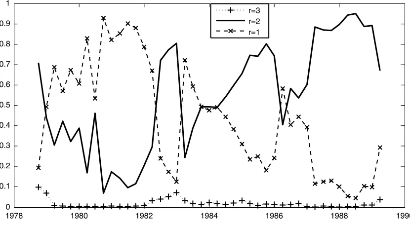
Before discussing the predictive power of money, we begin by summarizing evidence on which models are supported by the data. In particular, we present the probabilities attached to the models in our recursive BMA exercise based on the real-time data. For each real-time period, the same three models almost always receive the vast majority of the posterior probability. These three preferred models differ in the number of cointe-grating relationships but all have the same lag length, p=1, and hence, we focus on the uncertainty about the number of cointegrating relationships.
Figure1plots the probability ofr=1,2, and 3 cointegrating relationships (the probability ofr=0 is approximately zero). Since the sample includes many financial innovations, micro-economic reforms, and persistent data inaccuracies, we do not attempt an economic interpretation of the number of cointegrat-ing relationships. The overall impression one gets from lookcointegrat-ing at Figure1 is that the number of cointegrating vectors varies over time: the degree of model uncertainty that confronted pol-icymakers in real time is substantial. It is rare for a single model to dominate (e.g., one value ofrhardly ever receives more than 90% of the posterior model probability), and the model with the highest probability varies over time. There is almost no ev-idence for three cointegrating relationships. Models with two cointegrating relationships tend to receive increasing probabil-ity with time. However, prior to 1982, there is more evidence forr=1. During the critical period in which monetary targeting was abandoned, during the mid 1980s, ther=2 andr=1 mod-els are often equally likely, with several switches in the identity of the preferred model.
Faced with this considerable real-time model uncertainty, it seems reasonable that monetary policymakers may wish to (im-plicitly or ex(im-plicitly) average over different models, as is done by BMA. However, if a policymaker ignores the evidence from less preferred systems, then a strategy of simply selecting the sequence of best models is possible. In our recursive exercise, the best model varies over time. So the commonly used frequen-tist approach of selecting a single model using the BIC, and then basing forecasts on MLE’s involves many shifts between ther=1 andr=2 specifications. Typically, the evidence in Figure1suggests the most preferred model received between 90% and 50% weight. For a couple of periods, the best model receives less than 50% weight.
Turning to the more structural approach where we restrict the long-run parameters to be those implied by the money demand relationship (the VEL models), it is clear that restricting atten-tion to specificaatten-tions withr=1 has a substantial impact on the empirical relevance of the models. Figure1demonstrates
Figure 1. Probability of various models.
that for much of our sample, the evidence rarely provides very strong support ther=1 specification. Even though ther=1 models were typically preferred before 1985, they received less that 90% of the posterior probability in nearly all periods. Dur-ing 1986—when monetary targetDur-ing was abandoned—the prob-ability that the restriction holds was roughly 50%. Ther=1 model receives less than 40% weight from 1987 to the end of the sample.
4.2 In-Sample Prediction
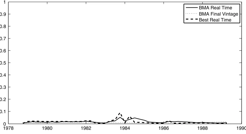
In this section, we examine the in-sample ability of money to predict inflation and output growth in our recursive exercise. Figure 2 plots the probability that money can predict output growth, and Figure3shows the corresponding plot for predict-ing inflation. All probabilities are calculated uspredict-ing the approach described in Section2. Each figure contains three lines. Two of these use the real-time data. The first of these lines uses BMA and the other uses the single model with highest probability— the best model. The third line uses the final vintage data, but we plot only BMA results. Hence, two of the lines use real-time data, and the third line has the advantage of hindsight. Results for the best model using final vintage data exhibit a similar pat-tern to BMA results, but are slightly more erratic and are omit-ted to clarify the graphs. The dates shown on thex-axis refer to the last observation for each vintage; these differ from the vin-tage date by the publication lag. So, for example, the 1986Q4 vintage has 1986Q2 as the last time series observation.
Figure2shows thatM3 has no predictive power for output growth, regardless of the model selection/averaging strategy or the type of data.M3, the preferred monetary target of U.K. poli-cymakers in this period, was phased out in 1989 where Figure2
ends.
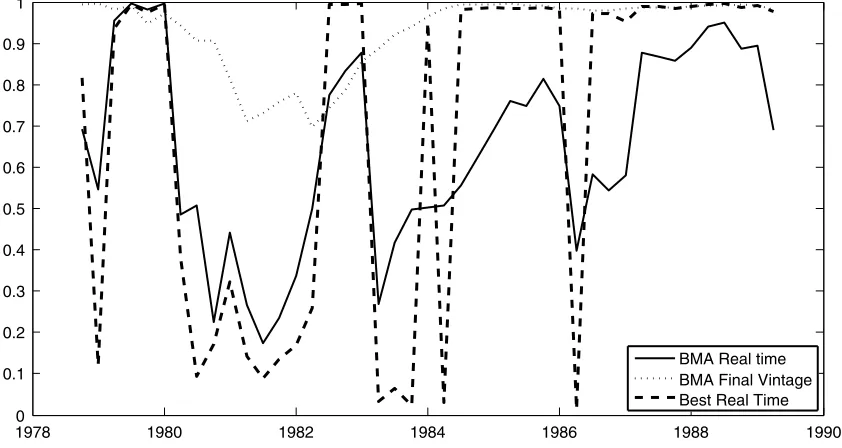
Figure3presents the probability that money has predictive power for inflation. The lines in this plot exhibit fluctuations. These are particularly pronounced for the best models with real-time data. The probability that money can predict infla-tion swings rapidly from near zero to near one several times
in the 1980s. A policymaker who simply selects the best model at each point in time could conclude that money mattered in some periods, but then next quarter it did not matter all. These switches between times when money matters, and when it does not, occur with embarrassing frequency.
Model averaging yields a less volatile pattern. In this case, there are repeated fluctuations, but the shifts in probability are not as sharp as with the best model selection strategy. The prob-ability that money matters for inflation increased for much of the 1980s, but there were quarters with rapid declines. In par-ticular, 1980 and 1984 saw distinct drops in predictability be-fore the official demise of monetary targeting in 1986. Further-more, in the last vintage in 1986, when the governor claimed predictability was causing difficulties with the monetary target-ing regime, the probability that money could predict inflation, using BMA and real-time data, fell to around 0.4 (plotted as 1986Q2) from approximately 0.8 in the previous quarter. We conclude that the real-time evidence in support of a relation-ship between money and inflation was prone to fluctuations.
With final vintage data, however, the BMA approach reveals no marked deterioration in the predictive power of money dur-ing the mid-1980s. The fluctuations in predictability discussed by the Governor of the Bank of England (Leigh-Pemberton
1986) are absent. Instead, following a fall to around 0.7 in the early 1980s, the probability that money matters for inflation rises back to approximately one by mid-1984. Comparing the real-time and heavily revised (final vintage) evidence, we con-clude that subsequent data revisions have removed the fluctua-tions in predictability that so concerned contemporary U.K. pol-icymakers in real time. The results presented in GKMV confirm that in-sample fluctuations in probabilities were not confined to theM3 monetary aggregate, the relationship with inflation, or the period of monetary targeting. Data revisions in the presence of model uncertainty caused large and repeated fluctuations in the predictability of money for other U.K. macro indicators.
The fluctuations with real-time data displayed in Figure3 re-sult from the changes in the model weights, plotted in Figure1.
Figure 2. ProbabilityM3 predicts output growth.
Figure 3. ProbabilityM3 predicts inflation.
The peaks and troughs in prediction probabilities almost ex-actly match the turning points forr=2 weights. The two coin-tegrating relationships system gives very high probabilities that money matters for inflation in almost all periods. The single long run relationship case suggests no relationship. (Hence, we have not plotted the VEL case in Figures2and3: the probabil-ities are zero for almost every period.)
It has been noted that using heavily revised data could dis-tort the predictive ability of broad money since data revisions might be aimed at strengthening the link between macroeco-nomic variables (see Diebold and Rudebusch1991, and Amato and Swanson 2001). There were minor changes to U.K. M3 during the 1980s (for example, due to the status of institutions recording money, and various privatizations). However, these small changes (typically smaller than 0.2% of the level) do not coincide with upwards movements in the probabilities reported in Figures2and3. It was not revisions to money, but rather re-visions to U.K. National Accounts that caused the divergence between the real-time and final vintage probabilities displayed in Figure3.
4.3 Out-of-Sample Prediction
Amato and Swanson (2001) argue that out-of-sample fore-cast performance should be used to judge the predictive content of money in real time. Although this approach is appealing in principle, small sample problems can make inference based on out-of-sample performance difficult in practice (see Clark and McCracken2006, and the references therein).
To illustrate the practical issues involved in real-time eval-uation of out-of-sample prediction, consider a monetary poli-cymaker evaluating the forecasting performance of our many models in 1986Q4. Publication lags for real-time data mean that the policymaker has time series observations up to 1986Q2. The lags between monetary policy implementation and other macro-economic variables imply that monetary policymakers are typ-ically concerned with predictions between one and two years
ahead. If the out-of-sample horizon of interest is 8 quarters from the last available observation, that is, 6 quarters ahead from the vintage date, the forecast of interest is for 1988Q2. Preliminary real-time outturns for this observation will only be released in the 1988Q4 vintage. Any changes in monetary policy at that date will have impacts roughly one to two years later—and by then, the U.K. business cycle has entered a differ-ent phase. A further complication is that the initial realizations of macroeconomic variables may not be reliable for forecast evaluations. Amato and Swanson (2001) argue that real-time forecasters should evaluate models using a number of vintages of outturns for real-time out-of-sample prediction, although this makes evaluations less timely.
With these issues in mind, and given the short sample of U.K. data available with theM3 definition of money, we limit our formal out-of-sample prediction analysis to using the final vin-tage for outturns. To be precise, we evaluate the performance of our predictions regardless of whether they are produced us-ing real-time or heavily revised (final-vintage) data by compar-ing them to the “actual” outcome. We use final vintage data for this “actual” outcome for the results presented (although we have experimented with other measures of “actual” outcome, discussed briefly below). We emphasize that these measures of predictive performance are not timely indicators—only a fore-caster with the 2006Q1 vintage (and the real-time dataset) could reproduce the tables reported in this section. Nevertheless, the ex post analysis provides insight into the out of sample perfor-mance of our models.
As in the previous section, we discuss the forecasting perfor-mance of different models, methodologies, and data sets. We compare the forecasting performance of theM3 system with money to the same system without money, using model aver-aging (BMA), the strategy of selecting the single best model (Best), and the structural approach (VEL). Separate sets of comparisons are made for real-time and final vintage data.
Technical details of the forecasting methodology are pro-vided in theAppendix. Suffice it to note here that, if pt+h
is our variable of interest (i.e., inflation in this instance or out-put growth,hperiods in the future), then we forecast using in-formation available at timet(denoted asDatat), where BMA
provides us with a predictive density Pr(pt+h|Datat)which
averages over all the models. This is what the BMA results be-low are based on. Our best model selection strategy provides us with a predictive density Pr(pt+h|Datat,MBest)whereMBestis
the model with the highest value for BIC. All of the features of interest in the tables below are functions of these predictive den-sities (i.e., point forecasts are the means of these denden-sities, etc.).
The structural results using the VEL models presented here use model averaging over ther=1 space (with some long-run para-meters fixed) using the methods outlined in Section2(selecting the best structural model gives similar results).
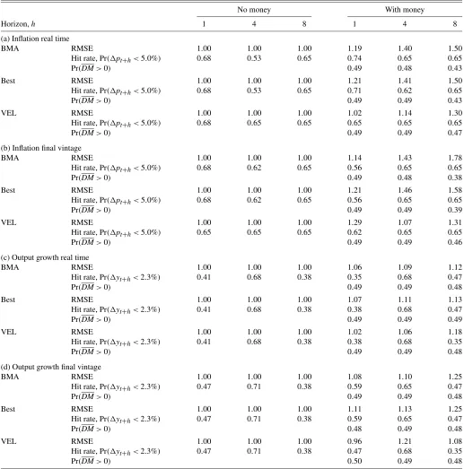
Table1presents results relating to the predictability of infla-tion and output growth for the M3 system. The upper panels (a) and (b) present results for inflation using real-time and final data, respectively; the bottom panels (c) and (d) present results for output growth using real-time and final vintage data, respec-tively.
Table 1. Evaluation of out-of-sample forecast performance
No money With money
Horizon,h 1 4 8 1 4 8
(a) Inflation real time
BMA RMSE 1.00 1.00 1.00 1.19 1.40 1.50
Hit rate, Pr(pt+h<5.0%) 0.68 0.53 0.65 0.74 0.65 0.65
Pr(DM>0) 0.49 0.48 0.43
Best RMSE 1.00 1.00 1.00 1.21 1.41 1.50
Hit rate, Pr(pt+h<5.0%) 0.68 0.53 0.65 0.71 0.62 0.65
Pr(DM>0) 0.49 0.49 0.43
VEL RMSE 1.00 1.00 1.00 1.02 1.14 1.30
Hit rate, Pr(pt+h<5.0%) 0.68 0.65 0.65 0.65 0.65 0.65
Pr(DM>0) 0.49 0.49 0.47
(b) Inflation final vintage
BMA RMSE 1.00 1.00 1.00 1.14 1.43 1.78
Hit rate, Pr(pt+h<5.0%) 0.68 0.62 0.65 0.56 0.65 0.65
Pr(DM>0) 0.49 0.48 0.38
Best RMSE 1.00 1.00 1.00 1.21 1.46 1.58
Hit rate, Pr(pt+h<5.0%) 0.68 0.62 0.65 0.56 0.65 0.65
Pr(DM>0) 0.49 0.49 0.39
VEL RMSE 1.00 1.00 1.00 1.29 1.07 1.31
Hit rate, Pr(pt+h<5.0%) 0.65 0.65 0.65 0.62 0.65 0.65
Pr(DM>0) 0.49 0.49 0.46
(c) Output growth real time
BMA RMSE 1.00 1.00 1.00 1.06 1.09 1.12
Hit rate, Pr(yt+h<2.3%) 0.41 0.68 0.38 0.35 0.68 0.47
Pr(DM>0) 0.49 0.49 0.48
Best RMSE 1.00 1.00 1.00 1.07 1.11 1.13
Hit rate, Pr(yt+h<2.3%) 0.41 0.68 0.38 0.38 0.68 0.47
Pr(DM>0) 0.49 0.49 0.49
VEL RMSE 1.00 1.00 1.00 1.02 1.06 1.18
Hit rate, Pr(yt+h<2.3%) 0.41 0.68 0.38 0.38 0.68 0.35
Pr(DM>0) 0.49 0.49 0.48
(d) Output growth final vintage
BMA RMSE 1.00 1.00 1.00 1.08 1.10 1.25
Hit rate, Pr(yt+h<2.3%) 0.47 0.71 0.38 0.59 0.65 0.47
Pr(DM>0) 0.49 0.49 0.48
Best RMSE 1.00 1.00 1.00 1.11 1.13 1.25
Hit rate, Pr(yt+h<2.3%) 0.47 0.71 0.38 0.59 0.65 0.47
Pr(DM>0) 0.48 0.49 0.48
VEL RMSE 1.00 1.00 1.00 0.96 1.21 1.08
Hit rate, Pr(yt+h<2.3%) 0.47 0.71 0.38 0.47 0.68 0.35
Pr(DM>0) 0.50 0.49 0.48
NOTES: RMSE denotes Root Mean Square Forecast Error, relative to the benchmark without money. The Hit rate is the proportion of correctly forecast events, with a correct forecast defined by the probability of the outturn greater than 0.5. The probability Pr(DM>0)is described inAppendix B.
We begin by discussing the results relating to inflation point forecasts. The rows labeled “RMSE” are the root mean squared forecast errors (where the forecast error is the actual realiza-tion minus the mean of the predictive distriburealiza-tion). All results are relative to the RMSE from BMA without money. A number less than one indicates an improved forecast performance rela-tive to this case (i.e., including money helps improve forecast performance). The general picture presented is that including money does not improve forecasting performance. These con-clusions hold regardless of whether we do BMA, select the best model, or take the structural approach.
Using the BMA predictive density, Pr(pt+h|Datat), we can
calculate predictive probabilities such as Pr(pt+h<a|Datat)
for any value ofa. Following Egginton, Pick, and Vahey (2002), we assume that the inflation rate prevailing when Nigel Lawson started as chancellor in July 1983 is the threshold of interest. Hence, for (GDP deflator) inflation we seta=5 percent. We de-fine a “correct forecast” as one where Pr(pt+h<a|Datat) >
0.5 and the realization is also less thana. The proportion of cor-rect forecasts is referred to as the “hit rate” and is presented in the tables.
An examination of Table1indicates that inclusion of money does improve some of the hit rates for inflation with real-time data, often by a substantial amount, at shorter horizons. For in-stance, the hit rate ath=4 with real-time data is 53% when money is excluded. However, when money is included the hit rate rises to 65%. In contrast, with final vintage data, the in-clusion of money causes little change in the hit rates, except at h=1.
In summary, we find some weak evidence that the inclusion of money has a bigger role in getting the shape and dispersion of the predictive distribution correct than in getting its location correct. That is, the RMSE results provided little evidence that including money improves point forecasts, but including money does seem to improve hit rates with real-time data (but not with final vintage data). Finally, it is worth mentioning that the hit rates are basically the same for BMA, the best single model and the VEL approach.
The row labeled Pr(DM>0)contains a Bayesian variant of the popular DM statistic of Diebold and Mariano (1995). De-tails are given inAppendix B. The basic idea is that we calcu-late a statistic which is a measure of the difference in forecast-ing performance between models with and without money. It is (apart from an unimportant normalization) the DM statistic. From a Bayesian point of view, this is a random variable, since it depends on the forecast errors which are random variables. If it is positive then models with money are forecasting better than models without money. Hence, if Pr(DM>0) >0.5 (that is a positive value ofDMis more likely than not) we find evi-dence in favor of of money having predictive power for inflation (output growth). As shown in Table1, we find no evidence that the inclusion of money improves forecast performance for in-flation. This statement holds true regardless of whether we are using BMA, selecting a single model or using the more struc-tural VEL models, and regardless of whether we are using final vintage or real-time data.
We turn now to output growth. In panels (c) and (d) of Ta-ble 1, we report the same set of forecast evaluation statistics for output growth. Our hit rates are based on the probability
Pr(yt+h<a|Datat)where we seta=2.3%, the average
an-nualized growth rate for the 1980Q1 to 2005Q3 period. The general conclusion is broadly similar to the inflation case: the RMSE does not improve when money is included. As with in-flation, there is a strong similarity of the RMSE results for the statistical strategies of BMA, selecting the single best models and using the structural approach VEL.
The same conclusion, that the inclusion of money makes rel-atively small differences, can be drawn from the hit rates. De-pending on the horizon, we see a slight worsening through to a slight improvement. For example, using BMA and real-time data, we see that including money worsens an already poor hit rate from 41% to 35% ath=1, stays the same at 68% forh=4, and improves from 38% to 47% forh=8. Using final vintage data and excluding money, the hit rates improve in two cases, but not forh=8. Including money has mixed impacts on final vintage hit rates: bothh=1 andh=8 have higher hit rates with money, but theh=4 case deteriorates.
Our Bayesian DM statistic provides more evidence for the story that including money does not improve output growth forecasts. For all of our models and approaches, the probability that this statistic is positive (that is, models with money have better forecast performance) is always very near to 0.5, indicat-ing roughly equal forecast performance between models with and without money.
We note that the performance of the various modeling ap-proaches and data types are typically robust to the alternative definitions of the outturn which we use to evaluate forecast performance. In Table 1, we use final vintage measurements as the “actual” outturn. For the sake of brevity, we do not in-clude results for other outturns (e.g., the first release outturn, or the outturn three years later). But results (available on re-quest) are very similar to those in Table 1. An exception to this is that the RMSE performance with money improves with first-release outturns. However, this exception is limited to the RMSE measure—beyond point forecasts, the results suggest that money does not matter.
The overall impression from our out-of-sample prediction analysis with theM3 monetary aggregate is that the system with no money provides a benchmark that is difficult to beat. For our short sample, there is little evidence that including money in the system makes substantial differences to out-of-sample pre-diction, either with real-time or final vintage data.
5. CONCLUSIONS
This paper investigates whether money has predictive power for inflation and output growth in the U.K. We carry out a recur-sive analysis to investigate whether predictability has changed over time. We use data which allow us to examine whether pre-diction would have been possible both in real time (i.e., us-ing the data which would have been available at the time the prediction was made), and retrospectively (using final vintage data). We consider a large set of VARs and VECMs which dif-fer in terms of lag length and the number of cointegrating terms. Faced with this model uncertainty, we use BMA. We contrast it to a strategy of selecting a single best model, and a more struc-tural approach motivated by a constant velocity money demand relationship.
Our empirical results are divided into in and out-of-sample components. With regards to in-sample results, using the real-time data, we find that the predictive content ofM3 fluctuates throughout the 1980s. However, the strategy of choosing a sin-gle best model amplifies these fluctuations relative to BMA. With BMA and final vintage data, the in-sample predictive con-tent of broad money did not fluctuate substantially during the 1980s. TheM3 monetary aggregate provides little help in pre-dicting output growth at any point. But we stress that results using final vintage data require the benefit of hindsight about data revisions. With the data that would have been available at the time, the salient feature is the fluctuations in the probability that money can predict inflation.
Our out-of-sample forecasting analysis suggests no strong evidence thatM3 matters for inflation or output growth, either with real-time or final vintage data.
U.K. policymakers have argued that fluctuations in the rela-tionships between broad monetary aggregates and inflation and output growth undermined their faith in the U.K.’s monetary tar-geting regime. The results in this paper indicate that they were right to worry about this issue. Issues relating to model uncer-tainty and data revisions have an important influence on beliefs about whether money matters.
APPENDIX A: PREDICTIVE DENSITIES FOR VARS AND VECMS
Let the VAR be written as
Y=XB+U, (A.1)
whereY is aT×nmatrix of observations on the n variables in the VAR.Xis an appropriately defined matrix of lags of the dependent variables and deterministic terms.Bare the VAR co-efficients andUis the error matrix, characterized by error co-variance matrix.
Based on theseT observations, Zellner (1971, pp. 233–236) derives the predictive distribution (using a common noninfor-mative prior) for out-of-sample observations,W generated ac-cording to the same model:
W=ZB+V, (A.2)
whereBis the sameBas in (A.1),Vhas the same distribution as U(see Zellner 1971, chapter 8 for details). Crucially,Z is assumed to be known. In this setup, the predictive distribution is multivariate Student-t(see page 235 of Zellner1971). An-alytical results for predictive means, variances, and probabili-ties such as Pr(pt+h<5.0|Datat)can be directly obtained
us-ing the properties of the multivariate Student-tdistribution. For other predictive features of interest, predictive simulation, in-volving simulating from this multivariate Student-tcan be done in a straightforward manner.
The previous material assumesZis known, which is straight-forward in the case of one period ahead prediction,h=1. That is, in (A.1), ifYcontains information available at timet, thenX will contain information datedt−1 or earlier. Hence, in (A.2) ifW is at+1 quantity to be forecast, thenZ will contain in-formation datedtor earlier. But for the case ofhperiod ahead prediction, whereh>1, thenZis not known. However, follow-ing common practice, we can simply estimate a different VAR
for each forecast horizonh. So forh=1 we can work with a standard VAR as described above, but forh>1, we can still work with a VAR defined as in (A.1), except letY contain in-formation at timet, but letXonly contain information through period t−h (i.e., let X contain lags of explanatory variables lagged at leasthperiods). In the notation used in the main text, for each forecast horizonh=1,2, . . . ,8 and recursion we esti-mate the following equation for output growth (or an equation for inflation) as part of our set of VECMs (VAR whenr=0) defined overpandr:
Leading the above equation byhtime periods givesyt+has
a function of known variables where their predictive densities will be multivariate Student-t and, hence, their properties can be evaluated (either analytically or simply by simulating from the multivariate Student-tpredictive density).
The preceding describes how we derivehstep ahead predic-tive densities for VAR models. The VECM can be written as in (A.1) if we include inXthe error correction terms (in addition to all the VAR explanatory variables). We replace the unknown cointegrating vectors which now appear inXby their MLEs. If we do this, analytical results for predictive densities can be ob-tained exactly as for the VAR. Note that this is an approximate Bayesian strategy and, thus, the resulting predictive densities will not fully reflect parameter uncertainty. We justify this ap-proximate approach through a need to keep the computational burden manageable. Remember that we have 80 models (i.e., 40 VARs and VECMs, each of which has a variant with money and a variant without money), and two different data combinations (i.e., we have real-time and final vintage versions of our vari-ables). For each of the different data combinations we have to do a recursive prediction exercise. Furthermore, we have to do all this forh=1,4, and 8. In total, our empirical results involve posterior and predictive results for tens of thousands of VARs or VECMs. Thus, it is important to make modeling choices which yield analytical posterior and predictive results. If we had to use posterior simulation, the computational burden would have been overwhelming.
APPENDIX B: A BAYESIAN VARIANT OF THE DIEBOLD–MARIANO STATISTIC
To develop a Bayesian interpretation of various frequentist ways of assessing predictive accuracy, consider the approach of Diebold and Mariano (1995). This involves comparing the predictive performance of two models (call them models 1 and 2). Their approach is based upon the forecast errors,e1tande2t
fort=1, . . . ,T for the two models. They letg(eit)fori=1,2
be the loss associated with each forecast and suppose interest centers on the difference between the losses of the two models:
dt=g(e1t)−g(e2t).
Diebold and Mariano derive a test of the null hypothesis of equal accuracy of the two forecasts. The null hypothesis is E(dt)=0. A test statistic they use is
T andvaris an estimate of the variance ofdused
to normalize the test statistic so that it is asymptotically N(0,1). From a Bayesian point of view, we will simply take dt as an
interesting feature useful for providing evidence on whether model 1 or model 2 is forecasting better. We will ignorevar (as it is merely a normalizing constant relevant for deriving fre-quentist asymptotic theory).
As a digression, it is worth noting that Diebold and Mari-ano’s method assumes there are two models. We are dealing with many more than that. However, this is simple to deal with in one of two ways. First of all, we can simply say model 1 is “the best model with money included” and model 2 is “the best model with money excluded” and then we do have two models, conventionally defined. However, when doing BMA it is valid to interpret “the BMA average of all models with money in-cluded” as a single model and “the BMA average of all models with money excluded” as a single model. This is what we do so in the relevant BMA rows of Table1.
Before beginning a discussion of a Bayesian analog to the DM statistic, we stress that the DM statistic depends on the forecast errors and, as used by Diebold and Mariano, is based on a point forecast. Our Bayesian methods provide us with point predictions and, thus, we could simply use theDMtest in ex-actly the same way as they do. Our statistical methods would then be a combination of Bayesian methods (to produce the pre-dictions) and frequentist methods (to evaluate the quality of the predictions). GKMV contains results using such an approach.
The fully Bayesian procedure used in this paper goes beyond point forecasts and treatseit as a random variable. That is, if
ytis the actual realized value of the dependent variable andy∗it
is the random variable which has the predictive density under modeli, then
eit=yt−y∗it
is a random variable anddtwill also be a random variable.
Re-member thaty∗
ithas at-distribution and, hence, if we treatytas
a fixed realization,eitwill also have at-distribution. Butdtis a
nonlinear function oft-distributed random variables and, hence, will not have a distribution of convenient form. Nevertheless, by using predictive simulation methods (i.e., drawingy∗it’s from thet-distributed predictive density and then transforming these draws as appropriate to produce draws ofdt) we can obtain the
density ofdtwhich we label
p(dt).
Remember that model 1 is better than model 2 [in terms of the loss functiong(·)] ifdt>0. So we can calculate
Pr(dt>0|Datat)
which will directly answer questions like “what is the probabil-ity that the model with money is forecasting better at timet?” If we average this over time
Pr(dt>0|Datat)
T
we can shed light on the issue “are models with money pre-dicting better overall than models without money?”. To make the notation more compact, in the text we label this Bayesian metric as Pr(DM>0).
In our empirical work, we use a quadratic loss function.
ACKNOWLEDGMENTS
We thank participants at the 2006 CIRANO Data Revi-sions Workshop, the 2007 FRB Philadelphia “Real-Time Data Analysis and Methods in Economics” conference, the 2007 CEF meetings, the Norges Bank Nowcasting Workshop 2007, and the Bank of Canada Forecasting Workshop 2007. We are grateful to Todd Clark, Dean Croushore, Domenico Gi-annone, Marek Jarocinski, James Mitchell, Serena Ng, Simon van Norden, Adrian Pagan, Barbara Rossi, Glenn Rudebusch, Yongcheol Shin, Tom Stark, Christie Smith, Norman Swanson, Allan Timmermann, and two referees for helpful comments. We acknowledge financial support from the ESRC (Research Grant RES-000-22-1342). The views in this paper reflect those of nei-ther the Reserve Bank of New Zealand nor Norges Bank. Alis-tair Cunningham (Bank of England) kindly provided the GDP data. Gary Koop is a Fellow at the Rimini Centre for Economic Analysis.
[Received August 2007. Revised August 2008.]
REFERENCES
Amato, J., and Swanson, N. R. (2001), “The Real-Time Predictive Content of Money for Output,”Journal of Monetary Economics, 48, 3–24.
Armah, N. A., and Swanson, N. R. (2007), “Predictive Inference Under Model Misspecification With an Application to Assessing the Marginal Predictive Content of Money for Output,” inForecasting in the Presence of Structural Breaks and Model Uncertainty, ed. M. Wohar, Amsterdam: Elsevier. Bachmeier, L. J., and Swanson, N. R. (2004), “Predicting Inflation: Does the
Quantity Theory Help?”Economic Inquiry, 43, 570–585.
Batini, N., and Nelson, E. (2005), “The UK’s Rocky Road to Stability,” Work-ing Paper 2005-020, FRB, St. Louis.
Bernanke, B., and Boivin, J. (2003), “Monetary Policy in a Data-Rich Environ-ment,”Journal of Monetary Economics, 50, 525–546.
Clark, T. E., and McCracken, M. W. (2006), “The Predictive Content of the Out-put Gap for Inflation: Resolving In-Sample and Out of Sample Evidence,”
Journal of Money, Credit and Banking, 38 (5), 1127–1148.
Cobham, D. (2002),The Making of Monetary Policy in the UK, 1975–2000, Chichester, U.K.: Wiley.
Corradi, V., and Swanson, N. (2006), “Predictive Density Evaluation,” in Hand-book of Economic Forecasting, eds. G. Elliott, C. W. J. Granger, and A. Tim-mermann, Amsterdam: North-Holland.
Corradi, V., Fernandez, A., and Swanson, N. R. (2009), “Information in the Revision Process of Real-Time Datasets,”Journal of Business & Economic Statistics, 27, 455–467.
Croushore, D., and Stark, T. (2003), “A Real-Time Data Set for Macroecono-mists: Does the Data Vintage Matter?”Review of Economics and Statistics, 85, 605–617.
Diebold, F. X., and Mariano, R. S. (1995), “Comparing Predictive Accuracy,”
Journal of Business Economics & Statistics, 13, 134–144.
Diebold, F. X., and Rudebusch, G. D. (1991), “Forecasting Output With the Composite Leading Index: A Real-Time Analysis,”Journal of the American Statistical Association, 86, 603–610.
Egginton, D., Pick, A., and Vahey, S. (2002), “Keep It Real! A Real-Time UK Macro Data Set,”Economics Letters, 77, 15–20.
Faust, J., Rogers, J., and Wright, J. (2005), “News and Noise in G7 GDP An-nouncements,”Journal of Money, Credit and Banking, 37, 403–420.
Feldstein, M., and Stock, J. H. (1994), “The Use of a Monetary Aggregate to Target Nominal GDP,” inMonetary Policy, ed. N. G. Mankiw, Chicago: Chicago University Press, pp. 7–62.
Fernandez, C., Ley, E., and Steel, M. (2001), “Benchmark Priors for Bayesian Model Averaging,”Journal of Econometrics, 100, 381–427.
Friedman, B. M., and Kuttner, K. N. (1992), “Money, Income, Prices and Inter-est Rates,”American Economic Review, 82, 472–492.
Garratt, A., and Vahey, S. P. (2006), “UK Real-Time Data Characteristics,” Eco-nomic Journal, 116, F119–F135.
Garratt, A., Koop, G., Mise, E., and Vahey, S. P. (2007), “Real-Time Prediction With Monetary Aggregates in the Presence of Model Uncertainty,” Working Paper 0714, Birkbeck, available athttp:// www.ems.bbk.ac.uk/ research/ wp. Garratt, A., Koop, G., and Vahey, S. P. (2008), “Forecasting Substantial Data Revisions in the Presence of Model Uncertainty,” Discussion Pa-per 2006/02, RBNZ;Economic Journal, 118, 1128–1144.
Inoue, A., and Kilian, L. (2005), “In-Sample or Out of Sample Tests of Pre-dictability: Which One Should We Use?”Econometric Reviews, 23, 371– 402.
Inoue, A., and Rossi, B. (2005), “Recursive Predictability Tests for Real-Time Data,”Journal of Business & Economic Statistics, 23, 336–345.
Johansen, S. (1991), “Estimation and Hypothesis Testing of Cointegrating Vec-tors in Gaussian Vector Autoregressive Models,”Econometrica, 59, 1551– 1580.
Leeper, E. M., and Roush, J. E. (2003), “Putting ‘M’ Back Into Monetary Pol-icy,”Journal of Money, Credit and Banking, 35 (2), 1217–1256.
Leigh-Pemberton, R. (1986), “Financial Change and Broad Money,”Bank of England Quarterly Bulletin, December.
(1990), “Monetary Policy in the Second Half of the 1980s,”Bank of England Quarterly Bulletin, November.
Orphanides, A. (2001), “Monetary Policy Rules Based on Real-Time Data,”
American Economic Review, 91, 964–985.
Orphanides, A., and Porter, R. (2000), “P* Revisited: Money-Based Inflation Forecasts With a Changing Equilibrium Velocity,”Journal of Economics and Business, 52, 87–100.
Roberds, W., and Whiteman, C. H. (1992), “Monetary Aggregates as Monetary Targets: A Statistical Investigation,”Journal of Money, Credit and Banking, 24 (2), 141–161.
Rudebusch, G. D., and Svensson, L. E. O. (2002), “Eurosystem Monetary Tar-geting: Lessons From US Data,”European Economic Review, 46 (3), 417– 442.
Schwarz, G. (1978), “Estimating the Dimension of a Model,”The Annals of Statistics, 6, 461–464.
Stock, J. H., and Watson, M. W. (1989), “Interpreting the Evidence on Money-Income Causality,”Journal of Econometrics, 40, 161–182.
(1999), “Forecasting Inflation,”Journal of Monetary Economics, 44, 293–335.
(2003), “Forecasting Output and Inflation: The Role of Asset Prices,”
Journal of Economic Literature, 41, 788–829.
Swanson, N. R. (1998), “Money and Output Viewed Through a Rolling Win-dow,”Journal of Monetary Economics, 41, 455–473.
Wroe, D. (1993), “Improving Macroeconomic Statistics,”Economic Trends, 471, 191–199.
Zellner, A. (1971), An Introduction to Bayesian Inference in Econometrics, New York: Wiley.