Full Terms & Conditions of access and use can be found at
http://www.tandfonline.com/action/journalInformation?journalCode=ubes20
Download by: [Universitas Maritim Raja Ali Haji] Date: 13 January 2016, At: 00:38
Journal of Business & Economic Statistics
ISSN: 0735-0015 (Print) 1537-2707 (Online) Journal homepage: http://www.tandfonline.com/loi/ubes20
Using Weights to Adjust for Sample Selection
When Auxiliary Information Is Available
Aviv Nevo
To cite this article: Aviv Nevo (2003) Using Weights to Adjust for Sample Selection When
Auxiliary Information Is Available, Journal of Business & Economic Statistics, 21:1, 43-52, DOI: 10.1198/073500102288618748
To link to this article: http://dx.doi.org/10.1198/073500102288618748
Published online: 01 Jan 2012.
Submit your article to this journal
Article views: 93
View related articles
Using Weights to Adjust for Sample Selection
When Auxiliary Information Is Available
Aviv
Nevo
University of California, Berkeley and the National Bureau of Economic Research (nevo@econ.berkeley.edu)
This article analyzes generalized method of moments estimation when the sample is not a random draw from the population of interest. Auxiliary information, in the form of moments from the population of interest, is exploited to compute weights that are proportional to the inverse probability of selection. The essential idea is to construct weights for each observation in the primary data such that the moments of the weighted data are set equal to the additional moments. The estimator is applied to the Dutch Transportation Panel, in which refreshment draws were taken from the population of interest to deal with heavy attrition of the original panel. It is shown how these additional samples can be used to adjust for sample selection.
KEY WORDS: Dutch Transportation Panel; General method of moments; Panel data; Refreshment samples.
1. INTRODUCTION
Sample selection arises when the observed sample is not a random draw from the population of interest. Failure to take this selection into account can potentially lead to inconsistent and biased estimates of the parameters of interest. This article develops a method that uses auxiliary information to inate the observed data so it will be representative of the population of interest; thus standard estimators applied to the weighted data will yield consistent and unbiased estimates.
Suppose, for example, that one wants to study a panel of individuals in which there is thought to be an unobserved individual-specic effect correlated with the independent vari-ables. Common solutions include “within” and rst-difference estimators. However, implementing these types of estimators requires at least two observations for each individual. If the panel also suffers from nonrandom attrition, then the subset of individuals observed for more than one period is no longer a random draw from the population of interest. Assume that additional samples are at our disposal that are representative of each of the cross-sections, but also suffer from attrition and thus do not allow consistent estimation of the parameters of interest. An example of such a dataset is the Dutch Trans-portation Panel (DTP) considered by Ridder (1992) and used herein.
The procedure proposed in this article suggests one possible way to use these additional samples, the refreshment samples. The refreshment samples are used to attach a weight to each observation in the balanced subpanel such that moments in the weighted sample are set equal to corresponding moments in the refreshment samples. Estimating the parameters of interest using standard panel estimators and the weighted balanced panel is proposed.
The proposed method exploits additional data to adjust for the selection bias by using it to estimate the selection proba-bility, the propensity score. Here the propensity score is used to inate the observations. This is not the only way to exploit the additional information. Alternatively, it can be used to construct a control function (Heckman 1979; Ridder 1992, for the data structure discussed later), to match observations (Ahn and Powell 1993), or to impute the missing observations
(Hirano, Imbens, Ridder, and Rubin 2001 for the data used herein).
The advantage of the proposed weighting method over the alternative methods of using the aforementioned additional information is its simplicity. Once the weights have been com-puted, the researcher can conduct the same analysis that he or she would perform if the data were randomly drawn from the population of interest, using the weighted data. Thus any esti-mator can be computed with little added complexity due to the selection. The weights can be computed either by setting up the problem as a standard generalized method of moments (GMM) problem, or by solving a linear programming prob-lem. The latter approach connects the proposed method to information-based alternatives to GMM.
Although the refreshment samples found in the DTP are not typical of economic data, the method proposed here is gen-eral. For example, census and annual surveys of manufactur-ers data are sources of random draws from the population of interest that can be matched with smaller datasets that suffer from attrition but have information on economic agents over time. Furthermore, the use of refreshment samples to adjust for selection bias motivates collection of such samples, a pro-cedure not often done.
1.1 Previous Literature
A survey of the literature on sample selection is beyond the scope of this article. (For this, see, e.g., Heckman 1979, 1987, 1990; Heckman and Robb 1986; Little and Rubin 1987; Newey, Powell, and Walker 1990; Manski 1994; Angrist 1995; Heckman, Ichimura, Smith, and Todd 1998; and references therein.) Nonetheless the aim is to relate the method proposed here to previous work. The use of weights to correct for sam-ple selection is not new to this article. For examsam-ple, many data-collecting agencies (including the U.S. Census Bureau)
©2003 American Statistical Association Journal of Business & Economic Statistics January 2003, Vol. 21, No. 1 DOI 10.1198/073500102288618748
43
provide sampling weights to correct for the sampling proce-dure. Manski and Lerman (1977) proposed a method for com-puting weights for choice-based samples (see also Cosslett 1981; Wooldridge 1999). In both of these examples, the selec-tion probability is known; in contrast, in this article the prob-ability of selection and the implied weights are estimated jointly with the parameters of interest. Methods that estimate the weights jointly with the parameters of interest also exist (e.g., Cassel, Sarndal, and Wretman 1979; Koul, Susarla, and Van Ryzin 1981; Heckman 1987).
The method proposed here differs from these methods in two ways. First, the weights are allowed to be a function of variables that are not fully observed in the main dataset, but for which some information is known through the additional moments. The weights are also allowed to be a function of the dependent variable. In other words, this is a nonignor-able selection mechanism (Little and Rubin 1987). Second, the weights are computed by exploiting auxiliary information. This connects the method proposed here to weighting tech-niques for contingency tables with known marginal distribu-tions (Oh and Scheruen 1983, sec. 3; Little and Wu 1991). These methods are extended by examining a logistic selection equation and by looking at regression functions rather than contingency tables.
The estimator used here can be related to information-theoretic alternatives to GMM (Back and Brown 1990; Qin and Lawless 1994; Imbens 1997; Kitamura and Stutzer 1997; Imbens, Spady, and Johnson 1998; Hellerstein and Imbens 1999). Standard GMM methods implicitly estimate the distribution of the data by the empirical distribution (i.e., giving each observation a density of 1/N 5. The information-theoretic alternatives use overidentifying moment conditions to improve on the estimates of the data distribution, by esti-mating the distribution jointly with the original parameters of interest. The focus of this literature has been on improv-ing efciency. A related work (Nevo 2002) has shown that the estimator proposed here can be related to these methods. The differences between the sampled population, from which the sample is drawn, and the population of interest are made explicit. Therefore, bias in the estimation of the distribution can be dealt with. It turns out that when the sampled popula-tion equals the target populapopula-tion, the estimator proposed here is equivalent to the one proposed by Imbens et al. (1998).
This article is organized as follows. Section 2 presents the proposed estimator, and Section 3 applies this estimator to the data used by Ridder (1992). Section 4 concludes.
2. THE MODEL AND PROPOSED ESTIMATOR
2.1 The Setup
Suppose that N independent realizations 8z11 z21 : : : 1 zN9
of a (multivariate) random variableZ with its support, , a compact subset of<P, are observed. In the population,Zhas a pdf,f 4Z5. Letˆü
1 denote the true value of the parameters of interest and letˆü
12ä1, whereä1 is a compact subset of< K.
Assumption A0. ˆ1üuniquely setE6–4Z1 ˆü157D0. Further-more, the moment function,–2 ä1! <
K, is twice continu-ously differentiable with respect toˆand measurable inZ, and E6–4Z1 ˆü
15–4Z1 ˆü1507andE6¡–4Z1 ˆ150¡ˆ017 are of full rank.
A way of estimating ˆü
1 would be to follow the analogy principle by choosing the estimate
O
ˆ1 s.t. 1 N
N
X
iD1
–4zi1ˆO15D00
Implicitly this assumes that the empirical distribution of the data is a consistent estimate off 4Z5. However, if the observed sample is not a random draw from the population of interest, then the foregoing estimate is biased and inconsistent.
Let DiD1 if and only if zi is fully observed. In a
cross-sectional context, DD0 could imply, for example, that the covariates are observed but the outcome variable is not. In a panel example, DD1 for the balanced subsample, whereas D D0 for individuals present only in some periods. From Bayes’s rule, the distribution of the observedziis
f 4Z—DD15Df 4Z5¢P 4DD1—Z5=P 4DD150
Assumption A1. P 4DD1—Z5is bounded away from 0. This assumption requires that any point in the support have a (strictly) positive probability of being observed. This is not a trivial requirement. Consider, for example, a truncation prob-lem, a type 1 Tobit model. A unit will be observed if and only if the dependent variable,y, exceeds a certain value. Because the conditioning vector, Z, includes the dependent variable, the selection probability,P4DD1—Z5, will equal either 0 or 1, depending on the value ofy. The proposed method will not be operational in such a case. If the correlation between the selection rule and the variable of interest is less than 1, then this assumption will be satised (e.g., the model considered in Heckman 1974).
Assumption A1 allows one to recover the pdf,f 4Z5, given knowledge off 4Z—DD15andP4DD1=Z5by
f 4Z5Df 4Z—DD15¢P4DD15=P4DD1=Z50 (1) Therefore,
E6–1 4Z1 ˆü157DZ –4z1 ˆü15f 4z5dz
DZ –4z1 ˆü15f 4z—DD15¢P 4DD15= P4DD1—z5dzD01
and the correct analog estimator becomes
O
ˆ2 s.t.
P 4DD15 N
N
X
iD1 1 P4DD1—zi5
–4zi1ˆO15D00 (2)
The empirical distribution of the selected sample can be used to consistently estimatef 4Z—DD15. Therefore, ifP 4DD1—Z5 is known, then (2) can be used to consistently estimate ˆ1. This is the fundamental idea behind using sampling weights to correct for nonrandom sampling in surveys and estimation in choice-based sampling (Manski and Lerman 1977; Cosslett 1981; Wooldridge 1999).
In general, the selection probability is unknown and must be estimated. To estimate the selection probability,P4DD1—Z5,
Nevo: Using Weights to Adjust for Sample Selection 45
exact knowledge of the expectation,hü, is assumed in the
pop-ulation of an R-dimensional function ofZ, denoted byh4Z5N . Formally, hü DE6h4Z57N DR N
h4z5f 4z5dz. Examples include
N
h4Z5DY, where the researcher knows the mean of the depen-dent variable, or h4Z5N DY¢X, where the researcher knows the (noncentered) covariance between the dependent variable and some of the independent variables. In the context of panel data, the moments hü can come from the moments of
the marginal (cross-sectional) distributional of the unbalanced panel. The application that follows demonstrates this.
Denoteh4Z5D Nh4Z5ƒhü. Note thatE6h4Z57D0. For now,
assume that these moments are known and defer a discussion of where they come from and the possibility that they are known with error. parameters. Note that by construction,
E£N
This section examines under what conditions the additional moments are sufcient to identify the selection probability. To see that the identication is not trivial, consider the fol-lowing example. LetZiD4Zi11 Zi25be a bivariate binary ran-dom variable, where Zit measures a characteristic (outcome)
of individuali in time t 4tD1125. Also, let DiD1 if i is
observed in both periods. If the attrition is nonrandom, that is, f 4Zi11 Zi256Df 4Zi11 Zi2—D1D15, then analysis based on the individuals observed in both periods will yield biased and inconsistent estimates. Equation (1) corrects this bias by using P4Di—Zi5 to weight the observations. Under what conditions is this probability identied?
In a large sample, the probabilitiesP4Zi1Dz11 Zi2Dz2—DiD
151 z11 z2280119can be estimated from the subsample of indi-viduals observed in both periods. Assuming that the original sample is a random sample from the population, the probabil-ityP 4Zi15can be identied. Suppose that additional informa-tion onP4Zi25 is available, for example, by taking a random draw from the population attD2. This additional information is not sufcient to identifyP 4Di—Zi5in general. Without infor-mation on either the joint probabilityP4Zi11 Zi25or additional restrictions, the selection probability is not identied.
This example demonstrates that even if the additional infor-mation comes in the form of the complete marginal distri-bution, identication is not trivial. If the additional infor-mation is in the form of marginal moments, this is even more true. Hirano, Imbens, Ridder, and Rubin (2001) proved that by assuming a particular functional form for the selec-tion probability, the probabilityP4Di—Zi5is identied (Hirano
et al. 2001, thm. 2). Because it is assumed that the additional
information comes in the form of moments, slightly different conditions are required for identication.
Assumption A2. The matrix E6h4Z5¢h4Z50—DD17 is of full rank.
Assumption A3. P4DD1—Z5Dg4h4Z50ˆ
25, whereg 22!
2is a known, differentiable, strictly increasing function such
that lima!ƒˆg4a5D0 and lima!ˆg4a5D1.
Most of the standard probability models satisfy assump-tion A3—in particular, the logisitic model of selecassump-tion used later, that isg4a5Dexp4a5=41Cexp4a55.
Proposition 1. Under assumptions A0–A3 and assuming that the functions h4¢5 can be constructed, the parameters ˆ D4ˆ11 ˆ25 are identied using a sample 8z11 z21 : : : 1 zN9,
such that zi for all i, are iid with the empirical distribution
converging tof 4z—DD15.
Proof. Assumptions A2 and A3 promise that the equations E6h4Z5=g4h4Z50ˆ
25—DD17D0 have a unique solution forˆ2 such thatˆ2Dˆü2. Therefore, under assumptions A0 and A1, the system of equations E6–4Z1 ˆ15=g4h4Z50ˆ25—DD17D0 has a unique solution for ˆ1 such that ˆ1Dˆ1ü. This and standard GMM theory (Hansen 1982; Newey and McFadden 1994) prove the proposition.
A necessary condition for identication is that the num-ber of (linearly independent) additional moments is at least as large as the number of parameters governing the selection, that is, the dimension of ˆ2. Assumption A3 requires more than this. The selection probability depends on the functions h4Z5, for which the expectation in the population is known.
2.3 Estimation
A three-step procedure is proposed for estimating the parameters of interest. In the rst step, the probability of selec-tion is modeled as
P4DD1—Z1 ˆ25Dexp4gü4Z1 ˆ255=41Cexp4gü4Z1 ˆ25551 (5) where gü4Z1 ˆ
25 is an unknown function. At this point no restrictions have been imposed, because ifgü4Z1 ˆ
25is dened appropriately, then (5) can t any selection model. The unknown functiongü4Z1 ˆ
25is approximated by a polynomial, h4Z50ˆ
2, with unknown coefcients,ˆ2. The model of selec-tion is driven largely by data availability, the presence of the functionsh4¢5. Assuming that a rich set of moments is avail-able for creating h4¢5, the model can be derived from eco-nomic modeling. In this case the estimates ofˆ2might be of independent interest.
The conditioning vector in (5) may also include the depen-dent variable in the estimation equation. Thus this selec-tion model is nonignorable. The selecselec-tion probability can be written as a function of observed variables as well as an individual-specic unobserved effect. Because the condition-ing vector includes the dependent variable in the main esti-mation equation, this type of selection model is covered by the setup in some cases, depending on the exact assumptions governing the distribution of the individual-specic effects.
The second step is to estimate weights that are proportional
By solving (6), the weighted sample counterpart ofE6h4Z57 is set to 0. Thus the additional moments, hü, are exploited
to estimate the parameters of the selection process. An alter-native interpretation of (6) comes from an information-based criterion. This interpretation relates the proposed method to information-theoretic alternatives to GMM (see the references listed in Sec. 1.1 and Little and Wu 1991). Details have been provided in earlier work (see Nevo 2002) for details.
Using gü4Z1 ˆ25Dh4Z50ˆ2 and substituting (5) into (6) yields the system of equations
N equation in the system dened by (7) will just be a normaliza-tion. Therefore, it can be ignored in the solution and imposed later by dividing all the weights by their sum. In such cases the parameter’ will not be identied separately from a scale parameter. The logistic selection probability proposed herein does not have this property. Thus this last equation will be more than just a normalization—it will actually change the relative weights. Consider, for example, a linear probability model, P4DD1—Z1 ˆ25DÁCZ0Â. The weights in such a case will be proportional to 6Á41CÁƒ10z0
iÂ57ƒ
1. Therefore, normalizing the weights to sum up to 1 will inuence only the estimate of the constant, not the relative weights. But if the probability of selection is logistic [i.e.,P4DD1—Z1 ˆ25D exp4h4Z50ˆ
25=41Cexp4h4Z50ˆ255] then, the weights will be proportional to 1Cexpƒ4ÁCz0
iÂ5. Now a normalization will
not be fully absorbed in the constant term and will inuence both the relative weights and their absolute value.
In the nal step, the weights that solve (6) are used to obtain analog estimates of the parameters of interest,ˆü
1. Formally, the estimate is given by
O
and the weights,wi, solve (6). The asymptotic properties of
this estimator are given by the following proposition.
Proposition 2. Suppose thatzi 4iD1121 : : : 5are iid with
the empirical distribution converging to f 4z—DD15, and (a)
assumptions A0–A3 are satised; (b)ä1ä2 is compact; (c) the moment functions,–4z1 ˆ5N , dened by (3), are twice con-tinuously differentiable inˆ; and (d) E6–4Z1 ˆ5N 0–4Z1 ˆ57 <N ˆ.
Proof. The expectation of the stacked moment conditions is set to 0 at the true parameter value; see (4). The assumptions of the proposition and standard GMM theory provide the result (Newey 1984; Pagan 1986; Newey and McFadden 1994).
The proof of the proposition stacks the moments as in (3) and considers them as just-identied estimation equations. The actual estimation can be obtained by solving these equations in one step (thus combining the second and third steps in the foregoing discussion.) However, as a computational issue, it is simpler to obtain the solution by rst solving (6), then plugging the solution into (8), as proposed in the foregoing algorithm. Given the assumptions and that the set of moments is just identied solving all the moments jointly or in two steps yields the same unique solution.
Alternatively, the standard errors can be estimated by boot-strapping. This works as follows. First, a bootstrap sample is generated by sampling from the original sample. Next, the value of the parameter that sets the moments in (3) to 0 is determined. These two steps are repeated to obtain the boot-strap distribution of the parameters.
The proposition assumes that the value of the population moments is known exactly. This seems to be an adequate assumption if the second dataset is much larger than the pri-mary dataset. However, in many interesting problems this will not be the case. Section 2.5 extends the results to take into account sampling error in the additional moments.
2.4 Examples of Data Structures
The proposed procedure assumes knowledge of population moments. A leading example of a source for these moments is the DTP used by Ridder (1992) and to which the pro-posed estimator is applied in Section 3. The unique design of this dataset called for draws of refreshment samples to deal with the heavy (seemingly nonrandom) attrition of the origi-nal panel. These refreshment samples are not characteristic of economic data. But, as the rest of this section demonstrates, under reasonable assumptions familiar economic datasets can t into the proposed framework.
Assume a combination of census data and smaller datasets (as in Imbens and Lancaster 1994; Hellerstein and Imbens 1999). The larger dataset can be viewed as a ran-dom draw from the population, which provides estimates of
Nevo: Using Weights to Adjust for Sample Selection 47
population moments for certain variables. The smaller dataset is not a random draw from the population of interest, however, it is much richer. For example, Gottschalk and Moftt (1992) documented the differences between the National Longitudi-nal Survey (NLS), a small and rich dataset, that suffers from attrition, and the Current Population Survey (CPS), which is not as rich, but is much larger and representative of the popu-lation. Hellerstein and Imbens (1999) exploited this to correct for ability in the NLS. The method proposed in this article, which is similar to their approach, suggests using the addi-tional data available from the CPS to treat the attrition in the NLS. The moments needed for the second step of the algo-rithm can be obtained from the CPS. The computed weights are then attached to the NLS, and the analysis is performed using the weighted dataset.
The data structure perhaps best suited for the proposed method is a panel structure. Consider the setup described in Section 1. The required moments,hü, can be obtained from
census data, which does not have a time dimension to it, as in the previous example. Alternatively, one might be willing to assume that each cross-section is a random draw from the marginal distribution of the population of interest, yet the bal-anced subsample is not a random draw from the joint distri-bution. As long as the probability of selection is a separable function of sectional variables, one can use the cross-sections to construct h4Z5. The parameters of interest can be estimated using standard panel estimators applied to the weighted balanced panel.
An example is the estimation of a production function. The rms observed at any given period can be considered a ran-dom draw from the population of potential rms. Yet, due to nonrandom exit and entry, restricting analysis to only those rms that existed in more than one period can potentially bias the results. (See Olley and Pakes 1996 for an example of the importance of accounting for entry and exit, and Griliches and Mairesse 1998 for a survey of the literature dealing with this problem.) The proposed method combines the full information contained in the unbalanced panel, while still controlling for the unobserved individual effects.
2.5 Taking Into Account Sampling Error in the Moment Restrictions
In the preceding sections, it was assumed that the additional information was in the form of exactly known moments,hü.
This is an adequate setup when the dataset providing these moments is much larger than the primary dataset; for exam-ple, if it is a census. However, in the example considered in Section 3, as in many other examples, this will not be the case. The results previously given can be generalized, as shown by Hellerstein and Imbens (1999), to the case wherehü
is not known with certainty but instead there is an estimate,
O
h, of hü based on a random sample of size M, that is, OhD
1=MPh4z
i5. This estimate satises
p
M 4Ohƒhü5 *N401 ã
h5,
withãhDE6h4z5¢h4z57. HereOhis assumed to be independent of the primary sample8z11 z21 : : : 1 zN9.
Nowˆcan be estimated by the algorithm described earlier, except nowhO instead ofhü is used to construct the additional
moments. This additional step must be taken into account
when investigating the properties of the estimator as the num-ber of observations in both datasets,N andM, goes to innity. If N =M converges to 0, then in large datasets the variance in the second dataset can be neglected, as in the case considered earlier. On the other hand, ifM =N converges to 0, then the second dataset cannot help adjust for sample selection. There-fore, this work considers only the case where the ratioM =N converges to a constantk.
The estimate of ˆ can be obtained by using the additional moments and standard GMM results. Without loss of general-ity, and to facilitate comparison with the previous exposition, assume thatM =N is exactly equal to some integerk. Let zQi
consist of8zi1 hn11 : : : 1 hik9. AssumeN observationszQ. Using the logistic selection probability, the estimating equations are
0D
of the estimators are the same as those produced by solving (7). The following proposition describes the asymptotic behav-ior of the estimator.
Proposition 3. Suppose that the conditions of Proposi-tion 2 hold; then the estimatorˆW
1 for ˆ1ü has the following
and ES6¢7 denotes expectations taken with respect to f 4z—DD15.
Proof. This is the same as the proof of Proposition 2 (see Hellerstein and Imbens 1999 for details).
3. AN EMPIRICAL APPLICATION
In this section the method described in the previous sections is applied to the DTP data used by Ridder (1992). Section 3.1 presents the data and initial analysis, and Section 3.2 gives the results based on the proposed procedure.
3.1 Data and Preliminary Analysis
The data are taken from the DTP, the purpose of which was to evaluate the change in the use of public transportation over time as price was increased. The rst wave of the panel con-sists of a stratied random sample of households in 20 towns interviewed in March 1984. Each member of the household, older than 11 years was asked to keep a travel log of all the trips taken during a particular week. A trip starts when the household member leaves the home and ends when he or she returns. Several questions were asked about each trip, but this information was not used here. (For a detailed description of the DTP, and a survey of research conducted with it, see van Wissen and Meurs 1990.)
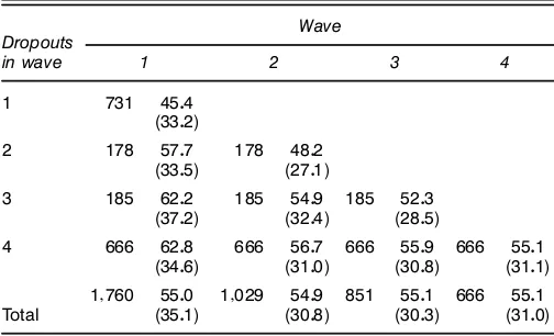
After the initial interview in March 1984, each participant who did not drop out was subsequently interviewed twice a year, in September and March. The September interviews did not ask the participants to ll out a detailed log and thus were somewhat different than the March interviews. This study fol-lows that of Ridder and examines only the March interviews (thus also avoiding any seasonal effects). The original panel suffered from heavy attrition, as seen in Table 1. To keep the number of participants constant, additional refreshment sam-ples were taken from the population. For the rest of this article it is assumed that the refreshments samples were taken as ran-dom samples from the population. In reality, the refreshment samples were sampled randomly with the same stratication as the original sample but with different weights, to compen-sate for the heavier attrition in some strata. The methods used here can easily deal with this case; however, for simplicity of presentation, this aspect is ignored. To demonstrate the pro-posed method, the focus is on explaining the number of trips taken as a function of household characteristics.
The average number of trips in different subsamples of the panel is given in Table 1. Examining the bottom row reveals that there is virtually no change in the average number of trips over the different waves. However, examining any one of the other rows shows a clear downward trend. This is not seen in the total, because the number of trips increases with the number of waves of participation. Surprisingly, these two effects completely offset each other.
Table 1. Number of Households and Average Number of Trips by Wave and Wave of Attrition
Wave Dropouts
in wave 1 2 3 4
1 731 4504
(3302)
2 178 5707 178 4802
(3305) (2701)
3 185 6202 185 5409 185 5203
(3702) (3204) (2805)
4 666 6208 666 5607 666 5509 666 5501
(3406) (3100) (3008) (3101)
11760 5500 11029 5409 851 5501 666 5501 Total (3501) (3008) (3003) (3100)
NOTE: For each wave, the left column presents the number of households and the right column presents the average number of trips and the standard deviation (in parentheses).
The data also contain information on various explanatory variables, described in the Appendix. The summary statistics demonstrate that the distribution of the variables differs in the different waves of the original panel. These differences in the distribution of the explanatory variables do not explain the pattern observed in the number of trips (Ridder 1992, table 5). This leaves (a combination of) the following as possi-ble explanations to the pattern in the number of trips observed in Table 1. Either there is a real downward trend in mobility or, due to nonrandom attrition, there are (nonrandom) differences in the distribution of the unobserved determinants of the total number of trips. Nonrandom attrition is a real concern given that the sample means of the variables in the waves of the original panel differ from the means in the refreshment panel. The question is whether this attrition completely explains the patterns of Table 1 or rather is part of the pattern due to a real change in mobility.
To answer this question, a series of regressions presented in Table 2 is computed. The following conclusions can be reached from the results in the table. First, if no correlation is assumed between the unobserved determinates of the num-ber of trips and the independent variables, then it can be con-cluded that there was no drop in mobility. This can be seen from the results in the rst two columns of the table, which are based on ordinary least squares regressions in the original sample plus the three refreshment samples. The three wave dummy variables are jointly statistically signicant at a 5% level. However, the dummy variables for the third and fourth waves are not jointly signicant. Therefore, it might be con-cluded that a drop in mobility occurred during the second period, but not overall.
Second, using the panel structure the assumption that unobserved household-specic effects are not correlated with the independent variables can be examined. The xed- and random-effects results can be combined to compute the stan-dard Hausman test, which is strongly rejected for both the bal-anced and unbalbal-anced panels (85.7 for the unbalbal-anced panel, 28.7 for the balanced panel). Therefore, it seems that the assumption made by the regression based on the repeated cross-sections is not valid, and that the estimates presented in the rst two columns are inconsistent. This also suggests that the only results in the table that are consistent are the within estimates, which point toward a large downward trend in mobility. If either the unbalanced or balanced panels are rep-resentative of the population, then it could be concluded that there was a downward trend in mobility. However, because it has already been demonstrated that the attrition from the sam-ple is nonrandom, this conclusion cannot be reached based on the results presented in any of the columns of Table 2.
Therefore, to determine whether there was a change in mobility we require an estimator that deals both with the attri-tion from the sample and the potential correlaattri-tion between the explanatory variables and the error terms. The estimator introduced in the previous sections has these properties and is used here. An additional estimator that could potentially deal with these issues is the one suggested by Hausman and Wise (1979). Ridder (1992) explored this estimator and found that it fails to alert of nonrandom attrition and hence also fails to treat it. Ridder attributed this failure to an implicit restric-tion that forces the covariance of the individual effects in the
Nevo: Using Weights to Adjust for Sample Selection 49
Table 2. Regression Results
Unbalanced panel Balanced panel
Repeated cross-sections
Variable OLS Total Within RE Total Within RE
Constant 55002 1091 3082 4066 7035 8093
(080) (1039) (1035) (1049) (1077) (2002)
Wave 2 ƒ3072 ƒ2092 ƒ4013 ƒ6057 ƒ5054 ƒ6025 ƒ5087 ƒ6007
(1054) (090) (079) (061) (057) (1007) (074) (073)
Wave 3 ƒ8039 ƒ064 ƒ5029 ƒ8018 ƒ7003 ƒ7081 ƒ7062 ƒ7072
(1068) (098) (084) (067) (061) (1007) (076) (073)
Wave 4 ƒ1072 ƒ1014 ƒ5004 ƒ8075 ƒ7041 ƒ8055 ƒ8037 ƒ8045
(1066) (096) (092) (075) (068) (1008) (080) (074)
Demographics No Yes Yes Yes Yes Yes Yes Yes
included
NOTE: The dependent variable is the total number of trips. White-robust standard errors are in parentheses. Except for the ’rst column, all regressions include as controls the demographic variables described in Table A.1.
selection and regression equations to have the same sign as the covariance of the random shocks in the two equations (see Ridder 1992, sec. 5, for details).
3.2 Results Using the Proposed Procedure
To evaluate the performance of the proposed procedure, two measures are examined. First, out-of-sample prediction of the model is studied by testing the ability of the weights, com-puted based on only the rst and last cross-sections, to match the weighted balanced panel moments with the moments from the refreshment panel. Next, estimates of the regression coef-cients are computed, similar to those presented in Table 2, which answer the question of whether or not there was a real change in mobility in the Netherlands.
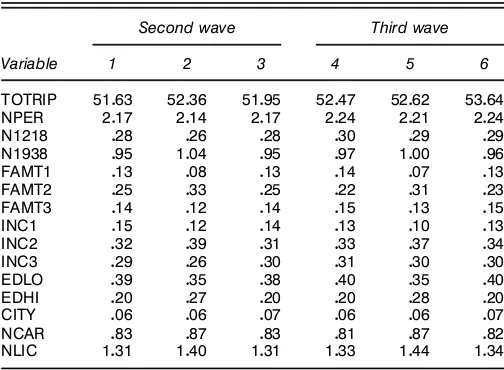
To test the out-of-sample predictive power of the methods, weights are computed by solving (7) using moments from the rst (unbalanced) wave of the panel and the last wave of the refreshment samples. Table 3 demonstrates the effects of weights on the sample statistics. Three different sets of weights were computed. The rst set was computed using moments on only the explanatory variables. This assumes a (particular) ignorable (conditional on observable variables) selection model. If selection is a linear function of only the explanatory variables, then these weights should control fully for selection. The second set of weights was computed using only the rst moments of the dependent variable (TOTRIP). Finally, all of the variables were used. In all cases, only the rst moments computed from the rst and last waves were used.
These weights were attached to the balanced observations, and the sample statistics for this weighted sample were com-puted. Table 3 presents the weighted sample averages for the second and third waves. Because the weights were computed using only the moments from the rst and fourth waves, these can be considered out-of-sample predictions. These moments can be used to construct a formal or informal test of the selec-tion model. Weights that control fully for selecselec-tion should ren-der the differences between the moments of Table 3 and the appropriate moments in Table A.2 as statistically insignicant.
The logic behind this is the same as that of the usual test of overidentication.
The results in Table 3 lead to the following conclusions. First, the weighted samples are more representative of the refreshment population, and thus of the population of interest. For all three selection models, the t is much better for the second wave than for the third wave. The ignorable selection model, which uses only the moments of the explanatory vari-ables, is quite strongly rejected. The third model, which uses both the dependant and independent variables, ts the second wave but not the third, suggesting that the third wave is some-what different.
One explanation of this last result can be seen by exam-ining different nonignorable models of selection. Under the model in which both the regression and selection equations are a function of xed (over time) individual-specic effects, selection should be fully controlled for by conditioning on the dependant variable. The difculty in predicting the moments in the third wave suggest that this model is wrong. Therefore,
Table 3. Weighted Sample Averages
Second wave Third wave
Variable 1 2 3 4 5 6
TOTRIP 51063 52036 51095 52047 52062 53064
NPER 2017 2014 2017 2024 2021 2024
N1218 028 026 028 030 029 029
N1938 095 1004 095 097 1000 096
FAMT1 013 008 013 014 007 013
FAMT2 025 033 025 022 031 023
FAMT3 014 012 014 015 013 015
INC1 015 012 014 013 010 013
INC2 032 039 031 033 037 034
INC3 029 026 030 031 030 030
EDLO 039 035 038 040 035 040
EDHI 020 027 020 020 028 020
CITY 006 006 007 006 006 007
NCAR 083 087 083 081 087 082
NLIC 1031 1040 1031 1033 1044 1034
NOTE: Weights are computed using in columns 1 and 4, ’rst moments of explanatory vari-ables in the ’rst and fourth waves; in columns 2 and 5, ’rst moments of TOTRIP in the ’rst and fourth waves; and in columns 3 and 6, ’rst moments of TOTRIP and all of the explanatory variables in the ’rst and fourth waves.
Table 4. Weighted Regression Results
Model 1 Model 2
Within Random effects Within Random effects
Variable Estimate SE Estimate SE Estimate SE Estimate SE
Constant 5017 1085 8011 1077
Wave 2 ƒ2012 069 ƒ2040 069 ƒ3042 072 ƒ2099 071
Wave 3 ƒ2010 069 ƒ2011 069 ƒ8001 074 ƒ6085 072
Wave 4 ƒ1077 071 ƒ1036 069 ƒ3041 077 ƒ2036 073
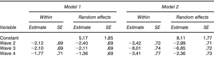
NOTE: The dependent variable is the total number of trips. In model 1 the weights are computed as a function of the dependent and independent variables in the ’rst and fourth waves (as in columns 3 and 6 of Table 3). In model 2 the weights are computed as a function of all the variables in wave 3 and the dependant variable in the other waves. All regressions include as controls the demographic variables described in Table A.1.
it is not surprising that Ridder (1992) found that the model of Hausman and Wise (1978), which makes these assumptions about the individual-specic effects, does not t this dataset. To deal with the poor t of the third-wave moments, the selec-tion probability is allowed to depend also on second- and third-wave variables.
Table 4 presents the weighted regression coefcients com-puted using the balanced panel. For each model, both a xed-effects estimator and a random-xed-effects estimator are computed. The models differ in selection probability. Model 1 models the selection probability as a function of the dependent and inde-pendent variables in the rst and fourth waves. It is equivalent to the selection model used to produce the results in columns 3 and 6 of Table 3. Because the analysis of the results in Table 3 suggests that this selection model does not fully capture the selection in the third wave, in model 2 the weights are com-puted as a function of all variables in the third wave and the dependent variable in the other waves.
The following conclusions can be drawn from the results. First, a Hausman test of the equality of the xed- and random-effects estimates is rejected. Despite this, the coefcients on the wave dummy variables are similar in both the xed- and random-effects models. Second, in general the weighted coef-cients are between the ordinary least squares results from the repeated cross-section and the (unweighted) balanced panel results. Finally, and most importantly, even after selection is controlled for in several different ways, the negative trend in mobility is still present. It is true that attrition makes this trend seem larger than it really is; however, it still exists. The drop in mobility is particularly large during the third wave. This is especially true in model 2, which allows for a more general model of selection in the third wave.
Given the count nature of the data, the foregoing analysis was repeated using a Poisson model for the number of trips. The only change was that the moments were now nonlin-ear in the parameters. The qualitative effects were similar to those found earlier. In particular, the estimates from a xed-effects (conditional) Poisson model suggest a downward trend in mobility, with a larger drop in the third wave. The esti-mates suggest that using model 2, the probability of taking a trip is reduced by about 5% in the second and fourth waves relative to the rst wave and is reduced by 15% in the third wave. Because the average number of trips is roughly 50, this is close to what the results of Table 4 imply.
4. FINAL REMARKS
This article proposes a weighting method that takes advan-tage of additional information to treat sample selection bias. Moments available from other sources are exploited to adjust for sample selection in the primary data. The method is appli-cable only in cases where these moments are available or can be estimated. Using these additional moments, the selection probability is computed, and this is used to inate the data. The estimator can deal with both ignorable and nonignorable selection mechanisms.
A few applications in which these additional moments are thought to be available have been out-lined. The application presented in detail is characterized by refreshment samples from the target population, which were taken to deal with attrition of the original sample. This is not typical of economic data, but perhaps it should be. Perhaps rather than putting great effort into maintaining panels that follow individuals or rms over a long period, more attention should be focused on obtaining additional cross-sectional draws from the population of interest.
An area for future work is a comparison of the method pro-posed here to alternatives. A full comparison, either theoreti-cal or empiritheoreti-cal, is beyond the scope of this article. However, some idea can be obtained by building on other work. Ridder (1992) used the same data reported used here to report results from a control function approach, as discussed earlier. The conclusions regarding mobility are similar to those obtained for the foregoing analysis. The same is true for an approach taken by Hirano et al. (2001) that involves imputing the miss-ing data. The method proposed here has one advantage over these two alternatives: It is much easier to implement. Com-puting the weights involves solving a simple system of equa-tions or, alternatively, a linear programming problem. It need be done only once, not repeatedly each time a new speci-cation of the main equation is examined. The actual analysis can be performed with the weighted data, applying standard methods and using standard software packets.
The last class of alternative methods is matching methods, in the spirit of Ahn and Powell (1993). This method does not use the auxiliary information discussed in this article, but it can be extended to do so. Such an extension would require different assumptions than those made in this article and is an interesting topic for future work.
Many public use datasets are accompanied by weights that are treated as known. The method proposed here allows the
Nevo: Using Weights to Adjust for Sample Selection 51
researcher to compute weights even if these are not avail-able or to compare the weights to the ones provided (because in some cases it is not clear how the provided weights are computed). However, even if weights are provided and the researcher is satised with how they were computed, there still might be an efciency argument for estimating the weights. Hirano, Imbens, and Ridder (2000) showed that in some cases estimators that weight observations by the inverse estimate of the selection probability are more efcient than estimators that use the true selection score. Furthermore, they related their result to the result of Wooldridge (1999) that shows that in the context of stratied sampling, it is more efcient to use esti-mated weights instead of known sampling probabilities. The MonteCarlo results of Nevo (2002) seem to suggest that a similar result might be applicable here.
ACKNOWLEDGMENTS
The author thanks Josh Angrist, Moshe Buchinsky, Francesco Caselli, Gary Chamberlain, Zvi Eckstein, Zvi Griliches, Jim Heckman, Kei Hirano, Guido Imbens, Jim Powell, and participants in the Econometrics in Tel-Aviv 1995 workshop and Camp Econometrics 1998 for useful discussions and comments on earlier versions of the manuscript, and Geert Ridder for making his data available.
APPENDIX: VARIABLES AND SAMPLE STATISTICS
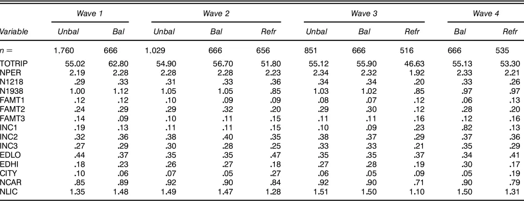
This appendix describes, the variables available in the data (Table A.1) and provides, their sample statistics in the different waves and subsamples (Table A.2).
Table A.1. The Explanatory Variables
Name Description
NPER Number of persons over age 11
N1218 Number of persons age 12–18
N1938 Number of persons age 19–38
INC1 Annual net family income<17,000 guilders INC2 Annual family income 24,000–37,999 guilders INC3 Yearly net family income 38,000 guilders CITY Inhabitant of large city (>500,000) NCAR Total number of cars in household
NLIC Total number of driving licenses in household FAMT1 Household with head under age 35 and no children FAMT2 Household with children younger than age 12 FAMT3 Household with head over age 65
EDLO Highest education of head primary school or lower EDHI Highest education of head university or higher
NOTE: From Ridder (1992).
Table A.2. Sample Averages of Variables
Wave 1 Wave 2 Wave 3 Wave 4
Variable Unbal Bal Unbal Bal Refr Unbal Bal Refr Bal Refr
nD 11760 666 11029 666 656 851 666 516 666 535
TOTRIP 55002 62080 54090 56070 51080 55012 55090 46063 55013 53030
NPER 2019 2028 2028 2028 2023 2034 2032 1092 2033 2021
N1218 029 033 031 033 036 034 034 020 033 026
N1938 1000 1012 1005 1005 085 1003 1002 085 097 097
FAMT1 012 012 010 009 009 008 007 012 006 013
FAMT2 024 029 029 032 020 029 030 012 028 020
FAMT3 014 009 010 011 015 011 011 016 012 016
INC1 019 013 011 011 015 010 009 023 082 013
INC2 032 036 038 040 035 038 037 029 037 036
INC3 027 029 030 028 025 033 033 021 035 029
EDLO 044 037 035 035 047 035 035 037 034 041
EDHI 018 023 026 027 018 027 028 019 030 017
CITY 010 006 007 005 027 006 005 009 005 019
NCAR 085 089 092 090 084 092 090 071 090 079
NLIC 1035 1048 1049 1047 1028 1051 1050 1010 1050 1031
NOTE: The columns labeledUnbal, Bal, andRefrpresent averages for the cross-section of the original panel, the balanced subpanel, and the refreshment samples.
[Received September 2000. Revised October 2001.]
REFERENCES
Ahn, H., and Powell, J. (1993), “Semi-Parametric Estimation of Censored Selection Models With a Non-Parametric Selection Mechanism,”Journal of Econometrics, 58, 3–29.
Angrist, J. (1995), “Conditioning on the Probability of Selection to Control Selection Bias,” Technical Working Paper 181, National Bureau of Eco-nomic Research.
Back, K., and Brown, D. (1993), “Implied Probabilities in GMM Estimators,” Econometrica, 61, 971–976.
Cassel, C., Sarndal, C., and Wretman, J. (1979), “Some Use of Statistical Models in Connection With the Non-Response Problem,”Symposium on Incomplete Data: Preliminary Proceedings.
Cosslett, S. (1981), “Maximum Likelihood Estimator for Choice-Based Sam-ples,”Econometrica, 49, 1289–1316.
Gottschalk, P., and Moftt, R. (1992), “Earnings and Wage Distributions in the NLS, CPS, and PSID,” Part I, Final Report to the U. S. Department of Labor, May 1992.
Griliches, Z., and Mairesse, J. (1998), “Production Functions: The Search for Identication,” inPracticing Econometrics: Essays in Method and Appli-cation, Cheltenham, U.K.: Elgar. Also inEconometrics and Economic The-ory in the 20th Century: The Ragnar Frisch Centennial Symposium, ed. S. Strom, Cambridge, U.K.: Cambridge University Press.
Hansen, L. (1982), “Large Sample Properties of Generalized Method of Moments Estimators,”Econometrica, 50, 1029–1054.
Hausman, J., and Wise, D. (1979), “Attrition Bias in Experimental and Panel Data: The Gray Income Maintenance Experience,”Econometrica, 47, 455–473.
Heckman, J. (1974), “Shadow Prices, Market Wages, and Labor Supply,” Econometrica, 42, 679–693.
(1979), “Sample Selection Bias as a Specication Error,” Economet-rica, 47, 931–961.
(1987), “Selection Bias and Self-Selection,” inThe New Palgrave: A Dictionary of Economics, eds. J. Eatwell, M. Milgate, and P. Newman, London: Macmillan Press, pp. 287–297.
(1990), “Varieties of Selection Bias,”American Economic Review, 80, 313–318.
Heckman, J., Ichimura, H., Smith, J., and Todd, P. (1998), “Characterizing Selection Bias Using Experimental Data,”Econometrica, 66, 1017–1098. Heckman, J., and Robb, R. (1986), “Alternative Methods for Solving the
Problem of Selection Bias in Evaluating the Impact of Treatments on Out-comes,” inDrawing Inferences From Self-Selected Samples, ed. H. Wainer, New-York: Springer-Verlag, pp. 63–107.
Hellerstein, J., and Imbens, G. (1999), “Imposing Moment Restrictions From Auxiliary Data by Weighting,”Review of Economics and Statistics, 81, 1–14.
Hirano, K., Imbens, G., and Ridder, G. (2000), “Efcient Estimation of Aver-age Treatment Effects Using the Estimated Propensity Score,” Technical Working Paper 251, National Bureau of Economic Research.
Hirano, K., Imbens, G., Ridder, G., and Rubin, D. (2001), “Combining Panel Data Sets With Attrition and Refreshment Samples,” Econometrica, 69, 1645–1659.
Imbens, G. (1997), “One-Step Estimators for Over-Identied General-ized Method of Moments Models,” Review of Economic Studies, 64, 359–383.
Imbens, G., and Lancaster, T. (1994), “Combining Micro and Macro Data in Microeconomic Models,”Review of Economic Studies, 61, 655–680. Imbens, G., Spady, R., and Johnson, P. (1998), “Information Theoretic
Approaches to Inference in Moment Condition Models,”Econometrica, 61, 655–680.
Kitamura,Y., and Stutzer, M. (1997), “An Information-Theoretic Alterna-tive to Generalized Method of Moments Estimation,”Econometrica, 65, 861–874.
Koul, H., Susarla, V., and Van Ryzin, J. (1981), “Regression Analysis With Randomly Right-Censored Data,”The Annals of Statistics, 9, 1276–1288. Little, R., and Rubin, D. (1987), Statistical Analysis With Missing Data,
New York: Wiley.
Little, R., and Wu, M. (1991), “Models for Contingency Tables With Known Margins When Target and Sampled Populations Differ,” Journal of the American Statistical Association, 86, 87–95.
Manski, C. (1994), “The Selection Problem,” inAdvances in Econometrics: Sixth World Congress, Cambridge, UK: Cambridge University Press, Vol. I, ed. C. Sims, 143–170.
Manski, C., and Lerman, S. (1977), “The Estimation of Choice Probabilities From Choice Based Samples,”Econometrica, 45, 1977–1988.
Nevo, A. (2002), “Sample Selection and Information-Theoretic Alternatives to GMM,”Journal of Econometrics, 107, 149–157.
Newey, W. (1984), “A Method of Moments Interpretation of Sequential Esti-mators,”Economics Letters, 14, 201–206.
Newey, W., and McFadden, D. (1994), “Estimation in Large Samples,” in The Handbook of Econometrics, North Holland: Amsterdam, Vol. 4, eds. D. McFadden and R. Engle.
Newey, W., Powell, J., and Walker, J. (1990), “Semiparmetric Estimation of Selection Models: Some Empirical Results,”American Economic Review, 80, 324–328.
Oh, H., and Scheuren, F. (1983), “Weighting Adjustments for Unit Non-Response,” in Incomplete Data in Sample Surveys, Vol. II: Theory and Annotated Bibliography, eds. W. Madow, I. Olkin, and D. Rubin, New York: Academic Press.
Olley, S., and Pakes, A. (1996), “The Dynamics of Productivity in the Telecommunications Equipment Industry,”Econometrica, 64, 1263–1297. Pagan, A. (1986), “Two Stage and Related Estimators and Their
Applica-tions,”Review of Economic Studies, 53, 517–538.
Qin, J., and Lawless, J. (1994), “Generalized Estimating Equations,” The Annals of Statistics, 22, 300–325.
Ridder, G. (1992), “An Empirical Evaluation of Some Models for Non-Random Attrition in Panel Data,”Structural Change and Economic Dynam-ics, 3, 337–355.
Van Wissen, L., and Meurs, H. (1990), “The Dutch Mobility Panel: Experi-ences Evaluation,”Transportation, 16, 99–119.
Wooldridge, J. (1999), “Asymptotic Properties of Weighted M-Estimators for Variable Probability Samples,”Econometrica, 67, 1385–1406.