Full Terms & Conditions of access and use can be found at
http://www.tandfonline.com/action/journalInformation?journalCode=ubes20
Download by: [Universitas Maritim Raja Ali Haji] Date: 12 January 2016, At: 01:07
Journal of Business & Economic Statistics
ISSN: 0735-0015 (Print) 1537-2707 (Online) Journal homepage: http://www.tandfonline.com/loi/ubes20
Sequential Causal Models for the Evaluation of
Labor Market Programs
Michael Lechner
To cite this article: Michael Lechner (2009) Sequential Causal Models for the Evaluation of Labor Market Programs, Journal of Business & Economic Statistics, 27:1, 71-83, DOI: 10.1198/ jbes.2009.0006
To link to this article: http://dx.doi.org/10.1198/jbes.2009.0006
Published online: 01 Jan 2012.
Submit your article to this journal
Article views: 148
View related articles
Sequential Causal Models for the Evaluation of
Labor Market Programs
Michael L
ECHNERProfessor of Econometrics, University of St. Gallen, Swiss Institute for Empirical Economic Research, Varnbuelstr. 14, CH-9000 St. Gallen, Switzerland (Michael.Lechner@unisg.ch)
This article reviews inverse selection probability weighting to estimate dynamic causal effects. A dis-tribution theory based on sequential generalized method of moments estimation is proposed and the method is applied to a reevaluation of some parts of the Swiss active labor market policy to obtain new results and discuss several issues about the implementation of the estimation procedure.
KEY WORDS: Causal effects; Dynamic treatment effects; Nonparametric identification; Panel data; Program evaluation; Sequential randomization.
1. INTRODUCTION
There is a substantial body of literature about the estimation of average ‘‘causal effects’’ of policy interventions using large micro data. Examples are numerous studies concerned with employment effects for unemployed who participate in pub-licly financed training programs. In this microeconometric framework, a causal effect is defined as a comparison of what would have happened in two (or more) different potential states of the world. This binary comparison is based on those observations that are actually observed in the two different states. If the allocation to a specific state is random, then the difference of the means of the outcome variables of the respective participants in the different states is a valid estimator for the average causal effect. If participation is not random, then selection problems arise and weighted means are required. In its static version, the selection problem received consid-erable attention in the microeconometric and statistics liter-ature, resulting in numerous suggestions about how to derive the required weights. Angrist and Krueger (1999); Heckman, LaLonde, and Smith (1999); and Imbens (2004) provide sur-veys of various parts of this vast literature.
However, the static model may not be able to address all relevant selection issues that may occur. Consider the evalua-tion of training programs: Suppose that interest is not in the effect of one particular training course, but in a sequence of courses. However, if the first course in such a sequence is effective, some unemployed individuals take up a job before the second course starts. If interest is not in the effect of the first course, but in the effect of the sequence of two courses, such behavior creates a selection problem that cannot be addressed in the static model. For example, solely controlling for pre-training variables does not work for obvious reasons. One important selection variable—namely, the outcome of the first participation—is missing. However, controlling for variables realized after the first training course that influence selection into the second course bears the potential problem that they may be influenced by the first part of the training sequence. Thus, they are ‘‘endogenous’’ and are ruled out as control variables in standard econometric approaches. Finally, it would be hard to find an instrument that is valid in that particular case. Robins (1986) suggests an explicitly dynamic causal framework that allows defining causal effects of dynamic interventions and systematically addressing this type of
selection problem. His approach is based on the key assump-tion that it is possible to control for the variables jointly influencing outcomes and selection at each particular selection step of the sequential selection process. Robins’ (1986) approach was applied subsequently in epidemiology and bio-statistics. Gill and Robins (2001) extend this approach to continuous treatments. Estimation strategies proposed for this model by Robins and various coauthors usually make para-metric or semiparapara-metric modeling assumptions about the relation of the potential outcomes to the confounding variables, like in g-estimation proposed by Robins (1986). G-estimation is based on recursively modeling the dependence of the out-come variables on the histories of confounders and treatments. To do so more parsimoniously, so-called ‘‘structural nested models’’ have been proposed by Robins (1993, 1994). How-ever, estimation (typically by some form of maximum like-lihood) of such models, which are necessarily complex, is very tedious. An alternative to this class of models are the so-called marginal structural models (MSM) again proposed by Robins (1998a, b). MSM are more tractable and probably more robust because they model the dependence of the potential outcomes only on those confounders that are time constant. Because controlling for those variables does not remove selection bias, weighting by the inverse of the treatment probabilities is used in addition. Robins (1999) discusses the advantages and dis-advantages of MSM and structural nested models. Various types of MSM are discussed in Robins, Greenland, and Hu (1999); Robins, Hernan, and Brumback (2000); Hernan, Brumback, and Robins (2001); as well as Joffe, Ten Have, Feldman, and Kimmel (2004). Miller et al. (2001) relate MSM to the literature on missing data problems. Estimation of MSM typically appears to be done by the (weighted) method of generalized estimating equations (Liang and Zeger 1986), which has conceptional similarities to the generalized method of moments (GMM) (Hansen 1982) that is more common in econometrics. So far, there seem to be no applications of dynamic potential outcome models to economic problems.
Lechner and Miquel (2001) adapt Robins’ (1986) framework to comparisons of more general sequences and different
71
2009 American Statistical Association Journal of Business & Economic Statistics January 2009, Vol. 27, No. 1 DOI 10.1198/jbes.2009.0006
parameters and selection processes, and reformulate the iden-tifying assumptions. The assumptions used by Robins et al. and Lechner and Miquel (2001) bear considerable similarity to the selection-on-observables or conditional independence assump-tion (CIA) that is prominent in the static evaluaassump-tion literature. When the CIA holds, inverse selection probability weighting (IPW) estimators as well as matching estimators are typically used (see Imbens 2004). Both classes of estimators have the advantage that the relation of the outcome variables to the confounders does not need to be specified. They require only the specification of the relation of the confounders to the selection process. In typical labor market evaluation studies, this feature is considered an important advantage, because applied researchers may have better knowledge about the selection process than about the outcome process. Although IPW estimators are, in principle, easy to implement and effi-cient under suitable conditions (e.g., Hirano, Imbens, and Ridder 2003), they are known to have problematic finite sample properties (e.g., Fro¨lich 2004) when very small or very large probabilities occur, which could lead to too much importance (weight) for a single (or a few) observations. However, although matching estimators may be more robust (but less efficient) in this sense, for many important versions of these estimators the asymptotic distribution has not yet been established (see Abadie and Imbens 2006).
This article proposes estimators for the models of Robins (1986) in the formulation suggested by Lechner and Miquel (2001) that retain the flexible and convenient properties of the aforementioned estimators, although some increase in com-plexity is unavoidable. Although sequential propensity score matching estimators could be applied in this context as well (and are presented in an earlier discussion paper version of this article that is available on the Internet), this article focuses on IPW estimation of the dynamic causal models. As mentioned earlier, it is an advantage that both methods do not require modeling the dependence of the outcomes and the confounders. The required specification of the relation between selection and confounders is done sequentially (i.e., each selection step over time is con-sidered explicitly), which allows a detailed and flexible speci-fication of this relation. Although these advantages are shared by both—matching and IPW estimators—it is easy to derive its asymptotic distribution only for IPW. For the case of a para-metric modeling of the relation of the selection process to confounders, in each period, which is the common case in static evaluation studies, this article provides the asymptotic dis-tribution of the IPW estimators based on the theory of sequential GMM estimation as proposed, for example, by Newey (1984). As a further addition to the literature in epidemiology, this article considers not only the estimation of the effects for some general population (the ‘‘average treatment effect,’’ as it would be called in the static evaluation literature), but also some effect of heterogeneity by treatment status (average treatment effects on the treated). Moreover, it discusses issues of common support that arise in this context with IPW estimation in some detail. An empirical analysis of different components of the Swiss active labor market policy illustrates its application and addresses a couple of practical issues.
The article proceeds as follows: Section 2 outlines the dynamic causal framework using the notation suggested by
Lechner and Miquel (2001), and details the IPW estimator. In Section 3, the practical application of the estimator is illustrated using Swiss administrative data. Section 4 concludes. Appendix A addresses issues that arise with multiple treatments as used in the empirical part. Appendix B shows the derivation of the sequential IPW estimator and its asymptotic distribution.
2. THE DYNAMIC CAUSAL MODEL: DEFINITION OF THE MODEL AND IDENTIFICATION
2.1 Notation and Causal Effects
This section briefly repeats the definition of the dynamic selection model as well as the identification results as presented by Lechner and Miquel (2001) using the terminology of the econometric evaluation literature. Because a three-periods– two-treatments model is sufficient to discuss most relevant issues that distinguish the dynamic from the static model and comes with a much lighter notational burden than the general model, this section shows the results only for this basic version. Suppose there is an initial period 0, in which everybody is in the same treatment state (e.g., everybody in the population of interest is unemployed), followed by two periods in which different treatment states could be realized (e.g., unemployed may participate in some training courses). Periods are indexed byt or t (t, t 2 {0,1,2}). For this population, the complete treatment is described by a vector of random variables,S¼(S1,
S2). A particular realization of St is denoted by st 2 {0,1}.
Denote the history of variables up to periodtby a bar below a variable, such as s2¼ ðs1;s2Þ: To differentiate between dif-ferent sequences, sometimes a letter (e.g.,j) is used to index a sequence, likesjt:As a further notational convention, uppercase
letters usually denote random variables, whereas lowercase letters denote specific values of the random variable. In the first period, a unit is observed in one of two treatments (partic-ipating in training,s1¼1; or not participating in training,s1¼ 0). In period 2, the unit participates in one of four treatment sequences {(0,0), (1,0), (0,1), (1,1)}, depending on what hap-pened in period 1. Therefore, every unit can participate in one sequence defined bys1and another sequence defined by the valuess1ands2. To sum up, in the two (plus one)-periods–two-treatments example, we consider six different overlapping potential outcomes corresponding to two mutually exclusive states defined by treatment status in period 1, plus four mutu-ally exclusive states defined by treatment status in periods 1 and 2.
Variables used to measure the effects of the treatment (i.e., the potential outcomes), such as like earnings, are indexed by treatments, and are denoted by Yst
t : Potential outcomes are
measured at the end of (or just after) each period, whereas treatment status is measured at the beginning of each period. For each length of a sequence (one or two periods), one of the potential outcomes is observable and is denoted by Yt. The
resulting two observation rules (called ‘‘consistency condition’’ by Robins 1986, or ‘‘stable unit value treatment assumption’’ by Rubin 1980) are defined in the following equation:
Yt¼S1Y1t þ ð1S1ÞY
0
t ¼S1S2Y 11
t þS1ð1S2ÞY
10 t
þ ð1S1ÞS2Y01t þ ð1S1Þð1S2ÞY 00
t ; t¼ 0;1;2:
Finally, variables that may influence treatment selection and potential outcomes are denoted by X. The K-dimensional vectorXt, which may contain functions ofYt, is observable at
the same time asYt.
Next, the average causal effect (for periodt) of a sequence of treatments defined up to period 1 or period 2 (t) compared with an alternative sequence us
k
Analogous to the static treatment literature, Lechner and Miquel (2001) callus
k
t;s
l
t
t the dynamic average treatment effect
(DATE). Accordingly,us DATE on the treated (DATET) and DATE on the nontreated, respectively. There are cases in between, like us
k
2;sl2
t ðsl1Þ, for which the conditioning set is defined by a sequence shorter than the ones defining the causal contrast, denoted by DATE(T). Note that the effects are symmetric for the same populationðuskt;slt exclude effect heterogeneityðus
k
of interest (with the same value ofs0) and is characterized by the random variablesðS1;S2;X0;X1;X2;Y1;Y2Þ:Furthermore, all conditional expectations of all random variables that are of interest shall exist. Under these conditions, Robins (1986) and Lechner and Miquel (2001) show that, if we can observe the variables that jointly influence selection and outcomes at each stage, then particular average treatment effects are identified. This assumption is called the ‘‘weak conditional independence assumption’’ (W-DCIA) by Lechner and Miquel (2001).
Weak Dynamic Conditional Independence Assumption
aÞ Y002 ;Y102 ;Y012 ;Y112 ‘S1jX0¼x0: dom variables B is independent of the random variable A
conditional on the random variableCtaking a value ofcin the sense of Dawid (1979). Part (a) of W-DCIA states that, con-ditional onX0, potential outcomes are independent of treatment choice in period 1 (S1). This is the standard version of the static CIA. Part (b) states that conditional on the treatment in period 1, on observable outcomes (which may be part ofX1) and on confounding variables of period 0 and 1ðX1Þ; potential out-comes are independent of participation in period 2 (S2).
To determine whether such an assumption is plausible in a particular application, we have to ask which variables influence
changes in treatment status as well as outcomes and whether they are observable. If they are observable, and if there is common support (defined in part (c) of W-DCIA, then we have identification, even if some or all conditioning variables in period 2 are influenced by the outcome of the treatment in period 1. To be more precise, the previously mentioned liter-ature shows that, for example, quantities like EðY112 Þ;
EðY112 jS1¼0Þ; EðY112 jS1¼1Þ; or E½Y211jS2¼ ð1;0Þ are
identified, but that E½Y112 jS2 ¼ ð0;0Þ or E½Y112 jS2¼ ð0;1Þ are not identified. Thus,us
k
sk1:This result states that pairwise comparisons of all sequences are identified, but only for groups of individuals defined by their treatment status in periods 0 or 1. The reason is that al-though the first period treatment choice is random conditional on exogenous variables, which is the result of the initial condition
S0¼0 for all observations, in the second period, randomization into these treatments is conditional on variables already influenced by the first period treatment. W-DCIA has an appeal for applied work as a natural extension of the static framework. Lechner and Miquel (2001) show that to identify all treat-ment parameters, W-DCIA must be strengthened by imposing that the confounding variables used to control selection into the treatment of the second period are not influenced by the selec-tion into the first treatment. Thus, the dynamic selecselec-tion problem collapses into a static selection problem with multiple treat-ments as discussed by Imbens (2000) and Lechner (2001a).
Appendix A contains some brief considerations for the dynamic case with multiple treatments. The extension to more than two periods is direct.
2.3 Estimation
All relevant estimators of the causal effects of the treatment sequences are based on differences of weighted means of the observable outcomes of those actually receiving the two treatments of interest:
i are the appropriate weights (‘‘^’’ indicates that
they are estimated).
An obvious way to reweight the observations of a specific treatment population toward the target populationðsj
tÞis to use the inverse of their respective selection probabilities of being observed in that treatment as opposed to the target population, following the ideas of Horvitz and Thomson (1952). Recently, the idea of directly reweighting the observations based on the choice probabilities has found renewed interest (e.g., Hahn 1998; Hernan et al. 2001; Hirano and Imbens 2001; Hirano et al. 2003; Nevo 2003; Robins, Hernan, and Brumback 2000; Robins and Rotnitzky 1995; Robins, Rotnitzky, and Zhao 1995;
Wooldridge, 2002, 2004). The reason is probably twofold. First, as advocated, for example, by Robins et al. (2000), they are easy to use, if a parametric model is used to estimate the choice probabilities. Second, Hirano, Imbens, and Ridder (2003) show for the static model, that for a suitably chosen nonparametric estimator of the choice probabilities, the inverse probability estimator is efficient.
Forsj
t¼s0;Robins et al. showed in various papers that the following weights lead to consistent estimators (empirical equivalent to the g-formula):
^ wsk2
i ¼
1
^ psk2jsk1
2 ðx1;iÞp^ sk
1
1ðx0;iÞ
8i2S2¼sk2; 8k:
^ ps
k
2jsk1
2 ðx1;iÞ denotes a consistent estimate of the transition
probability PðS2 ¼sk2jS1¼sk1;X1 ¼x1;iÞ and p^ sk
1
1ðx0;iÞ is a
consistent estimate of PðS1¼sk1jX0¼x0;iÞ: A similar result
can be derived for the DATE(T)—namely,
^ wsk2;s
j
1
i ¼
^ ps
j
1
1ðx0;iÞ
^ psk2jsk1
2 ðx1;iÞ^p sk
1
1ðx0;iÞ
8i2S2¼ sk2; 8k;j:
Appendix B shows that such weights solve the selection problem.
It is, so far, common practice in the static evaluation liter-ature to estimate such selection probabilities with parametric binary or multiple-response models (for each selection or transition). Under the standard regularity conditions of GMM estimation that are usually considered to be weak (see Hansen 1982 or, for this special case Newey 1984), such an estimator isffiffiffiffi
N
p
—consistent with an asymptotically normal distribution. Appendix B shows its asymptotic covariance matrix.
3. AN EMPIRICAL APPLICATION
In this section, the IPW estimator is applied to an evaluation of active labor market programs in Switzerland to show that it can provide interesting new insights, and discusses issues of implementation that may arise.
3.1 Setting the Scene
The study by Gerfin and Lechner (2002) serves as an example for this exercise. They are interested in the effects of different components of the Swiss active labor market policy on sub-sequent labor market outcomes using a rich administrative database coming from the merged records of the Swiss unem-ployment insurance system and the public pension system. They consider several types of programs and argue extensively that the data are informative enough to make the CIA plausible. Their study contains very good information about variables explaining program participation as well as potential outcomes, such as long employment histories; regional, sociodemo-graphic, and occupational information; as well as subjective information on the unemployed provided by the caseworkers who are in charge of program assignment. For more details about the programs evaluated and the data used, see Gerfin and Lechner (2002). This application relies on the same population as Gerfin and Lechner (2002), but uses the extended version of the sample described in the follow-up study by Gerfin, Lechner, and Steiger (2005).
Gerfin and Lechner (2002) estimate the effects of starting the first program in an unemployment spell. They focus on the beginning of the first program, because in a static model there are two endogeneity problems. First, any timing of the outcome measurement related to the end of the program may already incorporate some program effects. Second, subsequent gram participation may depend on the effect of the first pro-gram. The dynamic causal framework allows going further and accounting for the endogeneity of program duration and sub-sequent participation.
Here, interest is in the effects of being two periods in dif-ferent states for individuals entering unemployment in the last quarter of 1997. The different states used are unemployment (U), participating in training courses (C) or employment pro-grams (E), and receiving temporary wage subsidies (T). A period is defined as an interval of two months. Given the usual duration of Swiss programs, a bimonthly period appears to be appropriate to capture the essential dynamics. Any bimonthly period during which an individual participates at least two weeks in a program (C, E, or T) is considered program participation. In the rare event of participation in two different programs during the same period, the individual is defined to participate in the longest of those programs. Treatment occurs between January and April 1998. For example, considering sequences like EE compared with CC allows assessing the effects of four months of employment programs compared with four months of courses. Obviously, this approach allows investigating the effects of program combinations as well—for example, by comparing CE with UU or EE. As another example, it is pos-sible to check the effect of waiting for future participation by, for example, comparing UC (or UCC) with CC. For the sake of brevity, only effects of the types CC, EE, TT, and UU are considered. Because W-DCIA is assumed to hold, we consider only effects for subpopulations defined by the treatment in the first period.
The outcome variables of interest are the probability of finding unsubsidized employment as well as monthly earnings between May 1998 and the end of the observation period in December 1999. If we believe in the validity of the identi-fication arguments of Gerfin and Lechner (2002) for the beginning of the first program, then the part of W-DCIA relating to the first period is no problem. When the inter-mediate outcomes that determine the selection in March are observable, then the part of W-DCIA relating to the second selection step is plausible as well.
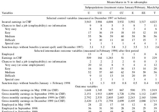
Table 1 gives descriptive statistics on some important control variables related to W-DCIA (see Table 2 for a full list of control variables used), treatments, and intermediate as well as final outcomes for the different subsamples of interest. The control variables (X0) considered in this table are the monthly earnings in the previous job, the subjective valuation of the caseworkers, as well as the number of sanction days without benefit (imposed by the caseworkers on unemployed individ-uals violating the rules). The subjective valuation gives an assessment of the employability of the unemployed. This assessment is a time-varying variable that the caseworker may change at the monthly interview of the unemployed (it is observed for every month). Comparing descriptive statistics across subsamples defined by treatment status reveals that
participants in employment programs are having the worst a priori chances in the labor market. Participants in temporary wage subsidies appear to be those with the best a priori chances. The lower panel in Table 1 shows statistics for the four intermediate outcomes (X1)—namely, employment, earnings, the subjective valuation of the caseworkers, and sanction days (i.e., reduced benefits if the unemployed violates the rules). Comparing the variables across treatments confirms the pre-vious conclusion. However, it also shows that participants leaving the sequence are different from participants who finish the sequence.
3.2. The Inverse Probability Weighting Estimator in Practice
3.2.1. Estimation of the Conditional Participation
Proba-bilities. Conditional probabilities are estimated at each step
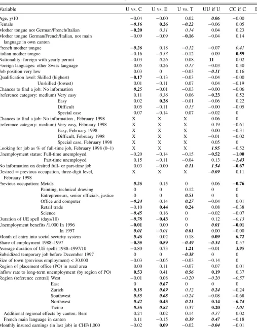
in each subsample using binary probits, which are subjected to specification tests. Table 2 presents the six binary probits that are required to estimate all selection equations that are of interest for the effects of the treatments defined earlier. The specifications broadly follow the specifications of Gerfin and Lechner (2002) and Gerfin et al. (2005) adjusted for the
spe-cifics of the dynamic framework, the different aggregation levels, and sample sizes. Because the outcome variables after period 1,X1, do not influence S1conditional on X0, they are omitted from the first period probits (their entries are denoted as X). Furthermore, the sample sizes and the variation of the dependent and independent variables in some cases require omitting specific variables from the specification (their entries are denoted as 0). The latter problem is particularly pronounced for the transition from E to EE, with only 19 observations leaving the sequence at this stage.
3.2.2. Common Support and the Sensitivity of the Inverse
Probability Weighting Estimator to Extreme Probabilities. It
may not be possible to obtain reliable estimates of the mean effects of the target populations as a whole, when some groups of the target population have characteristics that make them very unlikely to appear in one (or both) of the sequences under consideration. If it is impossible for such groups to appear in one of the treatments, then the support assumption of W-DCIA is violated, which means that the data are uninformative about this part of the target population (other than by extrapolation from other parts of the population). The common remedy is to remove this subpopulation from the target sample and redefine the causal effect appropriately. Even if their probability of Table 1. Descriptive statistics of control variables and intermediate outcomes
Variables
Means/shares in % in subsamples
Subpopulations (treatment status January/February, March/April 1998)
U UU C CC E EE T TT
Selected control variables (measured in December 1997 or before)
Insured earnings in CHF 3,943 3,904 4,008 3,932 3,592 3,517 4,023 4,067 Chances to find a job (employability): no information 9 8 5 5 8 7 11 14
Very easy 8 8 6 5 3 4 6 6
Easy 17 16 19 18 10 12 18 18
Medium 55 56 59 60 58 58 56 54
Difficult 9 10 11 10 17 15 7 7
Special case 1 1 1 1 4 4 1 2
Sanction days without benefits (current spell; until December 1997) 3.1 3.2 3.8 3.2 3.5 3.3 2.6 2.3 Selected intermediate outcome variables (measured in February 1998) after first period
Employed 13 4 2 1 1 0 6 1
Earnings in CHF 509 164 1,283 51 33 0 229 30 Chances to find a job (employability): no information 2 2 2 2 0 0 3 3 Very easy (or some employment) 20 12 8 5 4 4 12 8
Easy 16 16 17 16 13 14 20 21
Medium 52 57 60 62 59 59 56 59
Difficult 9 11 13 14 20 19 7 7
Special case 1 2 1 1 3 4 1 1
Sanction days without benefits JanuaryþFebruary 1998 1.2 1.3 0.9 0.8 0.5 0.4 0.5 0.6 Outcome variables
Gross monthly earnings in May 1998 (in CHF) 1,648 1,345 987 867 590 371 1,919 1,368 Gross monthly earnings in September 1998 (in CHF) 2,151 1,913 1,809 1,728 1,356 1,112 2,407 2,124 Gross monthly earnings in September 1999 (in CHF) 2,792 2,533 2,805 2,683 2,243 2,163 3,046 2,921 Gross monthly earnings in December 1999 (in CHF) 2,420 2,171 2,758 2,699 2,105 2,068 2,713 2,595 Employed in May 1998 28 22 17 14 12 8 29 22 Employed in September 1998 36 31 30 28 28 25 39 35 Employed in September 1999 49 44 49 46 40 39 52 52 Employed in December 1999 40 36 44 42 37 37 45 46 Sample size 7,985 5,122 573 316 118 99 790 382
NOTE: The sample is based on the selection criteria of Gerfin and Lechner (2002), but is constrained to those entering unemployment in the fourth quarter of 1997. The sequences are defined on a bimonthly basis. The states in each period are abbreviated as U (unemployed), C (training course), E (employment program), and T (temporary wage subsidy).X(XX) means being unemployed at the end of 1997 and in stateX(XX) for the first 2 (4) months in 1998 (X¼U, C, E, T).
Table 2. Probit specifications and coefficient estimates
Variable U vs. C U vs. E U vs. T UU if U CC if C EE if E TT if T
Age, y/10 0.04 0.00 0.02 0.06 0.00 0.44 0.00
Female 0.16 0.26 0.22 0.06 0.05 0.02 0.17
Mother tongue not German/French/Italian 0.20 0.31 0.14 0.04 0.23 0 0.11
Mother tongue German/French/Italian, not main language in own canton
0.09 0.09 0.16 0.04 0.14 0.16 0.19
French mother tongue 0.26 0.18 0.12 0.07 0.41 0.65 0.25
Italian mother tongue 0.16 0.33 0.12 0.09 0.59 0 0.03
Nationality: foreign with yearly permit 0.03 0.26 0.08 11 0.02 0.40 0.03
Foreign languages: other Swiss language 0.05 0.26 0.13 0.03 0.30 1.14 0.06
Job position very low 0.03 0 0.03 0.11 0.16 0.58 0.02
Qualification level: Skilled (highest) 0.17 0.13 0.03 0.04 0.00 1.11 0.22
Unskilled (lowest) 0.01 0.11 0.07 0.04 0.19 0.62 0.00
Chances to find a job: No information 0.25 0.01 0.03 0.00 0.06 0 0.37
(reference category: medium) Very easy 0.11 0.36 0.06 0.23 0.52 0 0.08
Easy 0.02 0.28 0.01 0.06 0.22 0 0.10
Difficult 0.05 0.11 0.13 0.00 0.05 0 0.15
Special case 0.07 0.14 0.07 0.02 0 0 0
Chances to find a job: No information , February 1998 X X X 0.06 0 0 0
(reference category: medium) Very easy, February 1998 X X X 0.19 0.61 0.32 0.05
Easy, February 1998 X X X 0.00 0.31 0.71 0.09
Difficult, February 1998 X X X 0.01 0.02 0.32 0.19
Special case, February 1998 X X X 0.05 0 0 0
Looking for job as % of full-time job, February 1998 (0–1) X X X 1.95 0.52 0.52 1.12
Unemployment status: Full-time unemployed 0.20 0.14 0.15 0.52 1.00 0.71 0.16
Part-time unemployed 0.15 0.11 0.04 0.13 1.43 0 0.38
No information on desired full- or part-time job 0.03 0.00 0.11 1.54 0.67 0 1.14
Desired¼previous occupation, three-digit level, February 1998
X X X 0.09 0.11 0.44 0.14
Previous occupation: Metals 0.26 0.15 0 0.06 0.76 0 0
Painting, technical drawing 0 0 0.12 0 0 0 0.33
Entrepreneurs, senior officials, justice 0 0 0.51 0 0 0 0.14
Office and computer 0.24 0.14 0.27 0.04 0.01 0 0.06
Retail trade 0.10 0.44 0.24 0.08 0.38 0 0.17
Science 0.45 0.16 0 0.02 0.07 0 0
Duration of UE spell (days/10) 0.78 0.43 0 0.12 0.13 0.05 0
Unemployment benefits /1,000 In 1996 0.01 0.00 0 0.01 0.01 0 0
In 1997 0.01 0.01 0.01 0.00 0.00 0.00 0.01
Month of entry into social security system 0.46 0.02 0.18 0.09 0.72 1.07 0.36
Share of employment 1988–1997 0.35 0.59 0.49 0.34 0.57 0 0.75
Average duration of UE spells 1988–1997/10 0.80 0.73 1.21 0.01 3.95 0 0.31
Subsidized temporary job before December 1997 0 0 0.38 0 0 0 0.19
Size of town (previous employment) < 30.000 0.03 0.05 0.03 0.14 0 0 0
Region of placement office (PO) in rural area 0.00 0.11 0.07 0.07 0.01 0.20 0.15
Inflow rate to long-term unemployment (by region of PO) 0.53 0.41 0.56 0.19 0.37 1.98 0.25
Region (reference central) West 0.01 0.08 0.20 0.20 0.57 0 0.06
East 0 0.67 0 0 0 0 0
Zurich 0.18 0.69 0.12 0.24 0.24 0.29 0.41
Southwest 0.55 0.68 0.24 0.08 0.68 0 0.13
Northwest 0.42 0.43 0.21 0.14 0.74 0.38 0.03
Ticino 0.56 0.82 0.37 0.20 1.01 0 0.19
Additional regional effects by canton: Bern 0.24 0.02 0.14 0.37 0.02 0 0.21
French main language in canton 0.11 0.15 0.39 0.47 0.18 0 0.13
Monthly insured earnings (in last job) in CHF/1,000 0.02 0.09 0.02 0.04 0.01 0.26 0.05
Employed February 2002 X X X 1.16 0.58 0 1.62
Current unemployment spell is first spell 0.02 0.01 0.12 0.07 0.31 0.80 0.07
Sanction days without benefits (current spell)/10 0.01 0.02 0.05 0.03 0.03 0.09 0.05
Sanction days without benefits/10, JanuaryþFebruary 1998 X X X 0.02 0.20 0 0.17
Subsample U or C U or E U or T U C E T
Number of observations in subsample 8,512 8,100 8,772 7,982 574 118 790
Dependent variable U U U UU CC EE TT
Mean of dependent variable in subsample 0.94 0.98 0.91 0.64 0.55 0.83 0.48
NOTE: Binary probit model estimated on the respective subsample. All specifications include an intercept and are subjected to specification tests (omitted variables, nonnormality). If not stated otherwise, all information in the variables relates to the last day in December 1997.Exclusion of variables: 0:Variables omitted from specification.X: Variable not temporarily prior to dependent variable. Bold numbers in italics denote significance at the 1% level. Bold numbers denote significance at the 5% level. Italics denote significance at the 10% level. See note in Table 1.
occurrence is positive but small, IPW estimators may have bad properties (e.g., Fro¨lich 2004; Robins et al. 2000; and the Monte Carlo study in the discussion paper version of this article). Therefore, even in this case the target population needs to be adjusted. Although, there is some discussion of support issues in the matching literature (e.g., Lechner 2001b; Smith and Todd 2005), the literature on IPW appears to be silent on that topic. The typical IPW solution to the problem is to remove (or rescale) observations with very large weights and check the sensitivity of the results with respect to the trimming rules used. Trimming observations, however, changes the target dis-tribution (shrinking large weights changes the target population as well, but in a way that is very hard to describe empirically). This change of the target distribution can be monitored by computing the same weights for the target population as for the treated population (i.e., the weights they would have obtained had they participated in such treatment). Then the sub-population with values of those probabilities that lead to a removal in one of the treatment samples is compared descrip-tively with the subpopulation with no such extreme values.
Because two potential outcomes are estimated for the same target population, trimming has to be done in both treated subsamples. However, when the trimming is done independ-ently for both subsamples, the estimates of the two mean potential outcomes may end up being valid for different target populations. Therefore, the same ‘‘types’’ of observations should be removed. Here, this idea is implemented in a simple way: Denote the weights used to weight observations in sequence 1 byw1i21 and those for observations in sequence 0 by w0i20: Compute both weights for the target population ðw0i2sj;w
1
i2sjÞ and both treatment populations ðw1i20;w0i21Þ as
well. Define the desired cutoff level for each treatment asw1
andw0:Reducew1ðw0Þto the largest value ofw1i20ðw0i21Þif it is below the originalw1ðw0Þ: This procedure could be iterated, but this was not necessary in the application. Based onw1and
w0, the target population is adjusted by considering only observations with values ofw0i2sjand w1i2sjless thanw1andw0:
Comparing descriptive statistics of confounders in the retained versus the deleted target sample shows how this reduction affects the interpretation of the parameters estimated. Furthermore, predicting the means of the confounders for the reduced sample in the same way as the mean potential outcomes is a second way to characterize the adjusted target population.
In the application, we compare the results of four different trimming rules for the various sequences and subpopulations. The first rule does not trim any observation at all; the second to fourth ones trim a given share of the observations with the largest weights (applied in both treated subsamples separately). The shares that are used are 0.1%, 1%, and 5%, respectively.
3.2.3 Results for the Different Estimators. Table 3
con-tains four blocks, with each block corresponding to an IPW esti-mator using one of the four cutoff rules. For each estiesti-mator, Table 3 contains a part related to common support issues (columns 3–6 and 12–15) and the weights (columns 7, 8, and 16, 17), as well as a part showing the estimates of the potential outcomes (monthly earnings in Swiss franks, CHF in December 1999; columns 5, 6 and 18, 19) and the effects of the sequences (columns 11, 20).
The part about the common support begins with the share of observations that would be deleted by adjusting the reference
distribution (column 3, 12). The deleted share increases with the decreasing cutoff points for the weights and it varies with the different sequences investigated.
Concerning trimming, using the 5% trimming leads to a loss of between 30% and 55% of the observations, whereas a .1% trimming rule leads to considerably smaller losses between 3% and 18%. Comparing different sequences, the largest losses occur when comparing participants in employment programs (EE) with recipients of temporary wage subsidies (TT). This is expected, because they are the most dissimilar groups.
The next column (4, 13) gives the mean of the earnings variable in the last job before treatment. This variable cannot be influenced by the treatment and is thus exogenous. Comparing its mean in the adjusted reference sample with its mean in the original reference sample (same as those for the IPW without trimming) shows the direction of the adjustment. With the exception of some comparisons based on the 5% rule, adjusting the reference distribution does not change the mean of this lagged earnings measure very much. Columns 5, 14 and 6, 15 contain the predictions of this variable based on the two treatment samples using the same weights as used for com-puting the mean potential outcomes. Because the effect for this variable is zero, those estimates should be similar (if the probability model is correctly specified) and both values should be similar to its mean in the adjusted reference population (column 4, 13). Taking into account the sampling variability, these conditions appear to be fulfilled. Thus, the comparisons, which are like balancing tests used with static matching, give no indication of a misspecification of the selection model used. Columns 7, 16 and 8, 17 contain the 10% concentration ratio of the weights in the two subsamples of treated observations (after adjusting for common support). This ratio shows the share of the target population covered by those 10% of the treatment population that have the largest weights. In the case of random assignment, this ratio would be about 10. However, if only a single observation is used to predict outcomes for all members of the target population, this ratio is 100. The results show systematically higher ratios when small treated groups are used to predict outcomes for large (and diverse) target populations, but overall do not indicate that the estimates are dominated by very few observations.
Columns 9, 18 and 10, 19 show the predicted counterfactual mean earnings of the sequences (1) for the respective target populations (2). Comparing the exogenous lagged earnings of both treatment groups with those of the target group using the lower panel of Table 1 gives an idea of whether we expect IPW to adjust mean observed posttreatment earnings upward or downward. Indeed, these adjustments appear to move the estimators in the expected direction in almost all cases.
Comparing the stability of the results across estimators (and thus across different common supports) shows qualitatively similar results, although the 5% trimming rule leads to a fairly different magnitude of the effect for the comparison of UU with CC for population U. In this case, the latter estimator finds considerably lower mean potential earnings for participating in CC compared with the other estimators. This goes along with the fact that when using the weights for the subpopulation in CC, the predicted mean lagged earnings are lower than the sample mean for the 5% rule, but are higher for the other
Table 3. Estimation results for gross monthly earnings (in CHF) in December 1999
Sequences
Target population
Common support
Concentration ratio of weights (in %)
Effects on current
earnings
Common support
Concentration ratio of weights (in %)
Effects on current earnings
E Ys2
t js1
% of target sample deleted
Mean ofY0
Predicted value of
E(Y0js1) % of
target sample deleted
Mean ofY0
Predicted value of E(Y0js1)
In adjusted target sample E Ys2
tjs1
In adjusted target sample
s12s02 s1 s1 s12 s02 s12 s02 s12 s02 u
s12;s02
t ð Þs1 s1 s12 s02 s12 s02 s12 s02 u
s12;s02 t ð Þs1
(1) (2) (3) (4) (5) (6) (7) (8) (9) (10) (11) (12) (13) (14) (15) (16) (17) (18) (19) (20)
IPW without adjustment IPW, 0.1% of largest weights removed
UU-CC U 0 3,943 3,912 4,048 16 42 2232 3,140 907 15 3,920 3,911 4,116 15 41 2,227 3,098 871
C 0 4,008 3,971 4,054 32 21 2,316 2,943 626 3 4,005 3,972 4,034 30 20 2,271 2,907 636
UU-EE U 0 3,943 3,911 3,912 17 46 2,232 1,971 260 18 3,844 3,822 3,666 16 42 2,207 2,166 41
E 0 3,592 3,557 3,598 42 18 2,037 2,076 39 5 3,532 3,497 3,558 42 18 2,014 2,118 103
UU-TT U 0 3,943 3,911 3,886 17 393 2,234 2,480 246 13 3,935 3,925 3,841 15 32 2,194 2,536 341
T 0 4,023 3,969 4,053 29 20 2,341 2,574 233 8 4,040 3,996 4,037 26 18 2,261 2,567 306
TT-EE T 0 4,023 4,053 4,165 19 48 2,592 2,047 545 16 3,941 3,978 3,827 18 40 2,500 2,361 139
E 0 3,590 3,624 3,598 45 18 2,313 2,076 237 10 3,581 3,604 3,613 44 17 2,249 2,161 88
IPW, 1% of largest weights removed IPW, 5% of largest weights removed
UU-CC U 22 3,925 3,926 4,065 14 37 2,231 2,991 759 44 3,966 3,972 3,904 13 30 2,307 2,692 385
C 9 3,985 3,989 3,987 31 21 2,293 2,848 555 30 3,895 3,945 3,914 29 19 2,281 2,731 449
UU-EE U 24 3,816 3,801 3,711 15 36 2,185 2,394 209 50 3,675 3,674 3,683 13 32 2,077 1,973 104
E 11 3,572 3,542 3,596 39 17 2,056 2,146 89 32 3,602 3,552 3,603 34 15 2,111 2,201 90
UU-TT U 17 3,940 3,947 3,813 14 29 2,179 2,454 274 30 3,992 3,998 4,005 13 24 2,198 2,458 260
T 14 4,037 3,998 4,034 25 16 2,257 2,620 362 30 4,018 4,026 4,005 22 15 2,284 2,590 305
TT-EE T 36 3,827 3,785 3,669 16 39 2,412 2,196 215 55 3,763 3,730 3,655 15 33 2,479 2,503 23
E 25 3,666 3,652 3,717 41 17 2,271 2,197 73 43 3,637 3,741 3,657 35 16 2,561 2,263 298
NOTE: Sequences: Treatments for which the effects are estimated.Target population: Population for which the effects of the treatments are estimated.Common support: Part of the target sample for which the effects could be estimated from observations in the two subsamples of treatment participants. In theadjusted target sample,observations for which the treatment sample could not be used to predict the effects are removed (the share of the removed part is shown in the column headed by ‘‘% of target sample deleted’’).Predicted value ofmeans that the mean ofY0is predicted using the same weights as used for the estimation of the effects.Concentration ratio of weights: Sum of the 10% largest weights divided by the sum of all weights3
100.Y0denotes insured monthly earnings in CHF (used by the unemployment insurance to calculate unemployment benefits). BecauseY0is computed from the UE insurance data, they may not be perfectly comparable with the outcome variable that is
calculated from the pension records.Earningsare coded as 0 if individuals receive a temporary wage subsidy, participate in a program, or are unemployed. For the effects, bold numbers in italics denote significance at the 1% level. Bold numbers denote significance at the 5% level. Italics denote significance at the 10% level. Estimates for the same counterfactual mean outcome may differ across different comparisons because the common support is comparison specific. See note in Table 1.
78
Journal
of
Business
&
Economic
Statistics,
January
estimators with more extreme cutoff values. This difference is reflected in the effect estimates as well. However, even though these differences exist, standard errors for the mean counter-factual are rather large. Therefore, it is probably not possible to reject the hypothesis that the estimators give the same results. Finally, it should be pointed out that, for several compar-isons, the number of observations ending up in the sequences is too small to lead to significant results, although the estimated effects are not too small (like for the comparison of UU with EE or EE with TT).
3.2.4. Effects of the Program Sequences on Labor Market
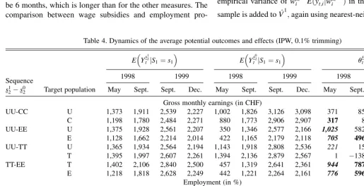
Outcomes. In addition to the result for December 1999, Table
4 presents results for outcome variables 1, 6, 17, and 20 months after the end of the sequence of interest to shed some light on the development of the effects over time. Furthermore, because it is the ‘‘official’’ objective for the active labor market policy to increase reemployment chances, in addition to the earnings variable that is shown in the upper panel of Table 4, an outcome variable measuring whether an individual is employed is pre-sented in the lower panel of Table 4.
To summarize, the results suggest that it is clearly better to participate in a course or receive a wage subsidy for two periods compared with remaining unemployed over that period. However, for employment programs it does not matter whether an unemployed person participates in such a program or remains unemployed. Of course, because the latter is much cheaper, employment programs appear to be ineffective. Looking at the dynamics of the program effects, the reason seems to be a large lock-in effect (individuals in the program search less intensively than those outside the program), because the typical duration of an employment program would be 6 months, which is longer than for the other measures. The comparison between wage subsidies and employment
pro-grams indicates the superiority of the former when both have at least a duration of two periods, but this effect is not estimated precisely enough for a firm conclusion.
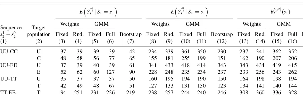
3.2.5. Standard Errors. Table 5 shows the results of five
different estimators for the standard errors. The first two pro-cedures shown in columns 3, 8, 13 and 4, 9, 14 are agnostic about the specific structure of the first-step estimator. They exploit the fact that the mean potential outcomes are weighted means of the observed outcomes in the respective sequence. To ease notation,
define normalized weights as w~s2k;s
j
t
i ¼ w^
sk
2;s
j
t
i
.P
iesk
2w^
sk
2;s
j
t
i : V^
1
estimates the variance conditional on the weights:
^
V1¼ varc X
iesk
2
~
ws
k
2;s
j
t
i yt;ijw^s
k
2;stj !
¼ X
iesk
2
~ ws2k;s
j
t
i
2 c
varyt;ijw^s2k;s
j
t
i
; jefk;lg:
The conditional variance of the outcome appearing in this term is estimated by a k-nearest-neighbor method. The number of neighbors is set to 2pffiffiffiffiN: There are robust to rather large changes in that smoothing factor, indicating that hetero-scedasticity conditional on the weights may not be a big issue in this application. Note that inference based onV^1 is
infor-mative about the effects defined for the sample, not the pop-ulation (see Abadie and Imbens [2006] for the distinction between population and sample treatment effects).
The second version acknowledges the randomness of the weights (var(A) ¼E(var(A|B) þ var(E(A|B)). Therefore, the
empirical variance of w~s2k;s
j
t
i E^ðyt;ijw^ sk
2;s
j
t
i Þin the respective
sub-sample is added toV^1;again using nearest-neighbor estimation
Table 4. Dynamics of the average potential outcomes and effects (IPW, 0.1% trimming)
E Ys 1 2 tjS1¼s1
E Ys 0 2 tjS1¼s1
us
1 2;s02 t ð Þs1
Sequence 1998 1999 1998 1999 1998 1999
s12s02 Target population May Sept. Sept. Dec. May Sept. Sept. Dec. May Sept. Sept. Dec.
Gross monthly earnings (in CHF)
UU-CC U 1,373 1,911 2,539 2,227 1,002 1,826 3,126 3,098 371 85 587 871
C 1,198 1,780 2,484 2,271 880 1,773 2,906 2,907 317 8 421 636
UU-EE U 1,375 1,928 2,561 2,207 350 1,346 2,577 2,166 1,025 582 15 41 E 1,128 1,662 2,214 2,014 422 1,165 2,179 2,118 705 496 34 104 UU-TT U 1,365 1,934 2,564 2,194 1,143 1,918 2,808 2,536 221 15 243 341 T 1,395 1,997 2,607 2,261 1,394 2,136 2,879 2,567 1 138 271 306
TT-EE T 1,402 2,106 2,840 2,500 457 1,319 2,641 2,361 944 787 199 139
E 1,218 1,818 2,628 2,249 442 1,221 2,264 2,161 776 596 364 88
Employment (in %)
UU-CC U 22 31 44 37 17 29 51 47 5 2 7 10
C 18 29 43 36 14 28 49 46 5 0 7 10
UU-EE U 22 32 45 37 7 30 51 39 16 2 5 2
E 19 29 41 35 8 26 37 37 11 3 4 1 UU-TT U 23 32 44 36 19 31 52 46 4 1 7 11
T 23 32 44 36 23 35 51 45 1 4 7 9
TT-EE T 24 35 52 46 9 30 44 38 15 5 8 9 E 22 33 51 44 9 28 40 37 13 6 12 7
NOTE: See notes in Tables 1 and 3.
to estimate the conditional expectation. Furthermore, because the observations in the different sequences are independent, the variance of the effect is computed as the sum of the variances of the potential outcomes. These estimators are in the same spirit as proposals by Abadie and Imbens (2006).
Because the parametric IPW estimators can be interpreted as sequential GMM estimators as, for example, analyzed by Newey (1984), the GMM approach is used to compute standard errors as well. Columns 5, 10, and 15 show the version that ignores the estimation of the probit coefficients, whereas the results in columns 6, 11, and 16 take full account of all random elements in the estimation process. All details on the GMM variances are presented in Appendix B.2.
Finally, columns 7, 12, and 17 present naive bootstrap esti-mates by taking the empirical standard deviation over the effects estimated in 1,000 random draws of 100% subsamples. Therefore, the bootstrap estimator is the only estimator that explicitly takes into account the variation that comes from the trimming rules.
Estimates are presented for the effects (columns 13–17) as well as for the potential outcomes (columns 3–7 and 8–12). Note that the estimation of the weights may induce a correla-tion between the outcomes, so that the variance of the effect does not necessarily equal the sum of the variances of the mean potential outcomes.
Comparing the estimates across the board, it is obvious that, for the larger treatment samples, all estimates are close together (level of UU for target population U, T, or E), whereas, for the smaller samples, they deviate much more from each other. It may be suspected that this results from less precise estimation of the variances in the smaller samples. In general, it is hard to detect any systematic trends, other than V^2 being
systemati-cally larger thanV^1(which must be the case by construction of
the estimators). Furthermore, in many casesV^1gives the smallest
variance. Comparing the two GMM estimators with each other, we see that, with five exceptions, taking into account the fact that the selection probabilities are estimated reduces the variance. This feature of IPW estimation has been frequently observed in the literature (see, for example, Hirano et al. 2003; Lunceford
and Davadian 2004; Robins et al. 1995; or Wooldridge 2002). Finally, the bootstrapped standard errors appear to be at the lower end of the values presented, which is somewhat surprising. However, it might be conjectured that the rule brings in some ‘‘nonsmoothness’’ that leads to a deviation from the validity of the bootstrap. However, it is beyond the scope of this article to investigate the issue of precise variance estimation of the IPW estimator in depth. Here, it suffices to see that the different estimators lead to similar statistical decisions for most cases.
4. CONCLUSION
This article discusses sequential IPW estimators to estimate mean causal effects defined within the dynamic causal model introduced by Robins (1986). GMM theory is used to provide a distribution theory for the case when the selection probabilities are estimated nonparametrically. Using an evaluation study of the Swiss active labor market policy, some implementational issues, like the so-called common support problem, are dis-cussed and results are provided. The application indicates that the dynamic approach allows investigating interesting ques-tions about causal effects of different regimes of active labor market policies. It also indicates that precise answers to these new questions require sufficiently large samples.
APPENDIX A: MULTIPLE TREATMENTS AND MANY PERIODS
The main issue concerns the specification of the propensity scores. For example, when specifying the probability of par-ticipating insk
2 conditional on participating in s1k, is it neces-sary to account for the fact that not participating insk
2 implies a range of possible other states in period 2? The answer is no, because in each step the independence assumption relates only to a binary comparison, such as Ys2k
2 ‘1 S2¼sk2
jS1 ¼
sk
1;X1¼x1, and Y sk
1
2 ‘1 S
1¼sk1
jS1e sj1;sk1
;X0¼x0ðsj1 being the target population as before). Therefore, the condi-tional probabilities of not participating in the event of interest Table 5. Asymptotic standard errors for gross monthly earnings (IPW, 0.1% trimming)
Sequence Target population
E Ys12 t jS1¼s1
E Ys02 t jS1¼s1
us12;s02 t ð Þs1
s12s02
Weights GMM
Bootstrap
Weights GMM
Bootstrap
Weights GMM
Bootstrap Fixed Rnd. Fixed Full Fixed Rnd. Fixed Full Fixed Rnd. Fixed Full
(1) (2) (3) (4) (5) (6) (7) (8) (9) (10) (11) (12) (13) (14) (15) (16) (17)
UU-CC U 37 39 39 39 42 234 339 361 350 230 237 341 362 352 231 C 48 58 56 77 65 155 181 255 199 151 162 190 207 206 152 UU-EE U 37 39 40 39 61 341 433 418 414 343 343 434 419 415 348 E 52 62 60 127 90 228 248 235 234 237 233 256 243 262 231 UU-TT U 35 37 37 37 50 160 195 194 190 150 164 198 198 194 155 T 42 49 48 67 51 127 133 131 130 123 134 141 140 144 129 TT-EE T 194 251 231 226 219 238 257 244 240 246 308 360 336 328 313 E 137 145 141 135 148 381 480 472 426 370 405 501 493 447 394
NOTE: See notes in Tables 1 and 3. Weights Fixed: Standard error of weighted mean estimator conditional on weights allowing for weight-dependent heteroscedasticity. Weights Rnd.: Standard error of weighted mean estimator allowing for weight-dependent heteroscedasticity and accounting for randomness of weights. GMM Fixed: Standard errors derived from GMM approach ignoring estimation of probabilities used to compute weights. GMM Full: Standard errors derived from GMM accounting for the estimation of the probabilities used to compute weights. Bootstrap: Standard deviation of 1,000 independent bootstrap estimates of the effects.
conditional on the history are sufficient, Imbens 2000 and Lechner 2001a, develop the same argument to show that, in the static multiple-treatment models, conditioning on appropriate one-dimensional scores is sufficient.) Hence, PðS2¼sk2jS1 ¼
sk1;X1¼x1Þ and P S1¼s1kjX0 ¼x0;S1e sl1;s1k
may be used to construct the weights. The multiple-treatment feature of the problem does not add to the dimension of the propensity scores.
APPENDIX B: THE SEQUENTIAL INVERSE PROBABILITY WEIGHTED ESTIMATORS
B.1 Nonparametric Identification
In this appendix, two examples show that the sequential inverse probability weighting (SIPW) estimators proposed in Section 2.3 are indeed estimating the desired quantities. For simplicity, it is assumed that the probabilities are estimated consistently and with enough regularity such that the following exposition based on true probabilities holds asymptotically with estimated probabilities as well.
a) The SIPW estimator forEðYs2k thermore, Bayes rule gives the connection between the conditional and unconditional counterfactuals. For
EðYs2k
B.2 Distribution of Two-Step Estimator with Parametric First Step
The previous section showed that the suggested sequential IPW estimator is nonparametrically identified. Here, the asymptotic distribution of the specific estimator used in the application is presented. It consists of estimating the weights in a first step without considering the outcomes. In the second step, the estimated weights are used to obtain the reweighted mean of the outcomes in the respective subsample. The general structure of the estimator is as follows:
^
and the estimated transition probabilities. Assume that these probabilities are known up to a finite number of unknown coefficients,b. Furthermore, assume that there is a consistent, asymptotically normal estimator of these coefficients, b^;
obtained by solving a number of moment conditions of the same dimension asb. These moment conditions are denoted by
gðx1;i;s2;i;bÞand have expectation zero at the true value ofb. The estimator for choosing the unknown values ofbfulfills the following condition:
For example, this would be the case if a probit model is used for the estimation of the various probabilities. In this case, the moment conditions correspond to the score of the likelihood function. Note that this moment condition is a collection of all moment conditions that are required to compute all necessary transition probabilities that enter the weight function. Thus,bis a collection of all parameters necessary to characterize the transition probabilities required for a particular weight function. To ease notation, rewrite the estimator of the effect in terms of a moment condition:
These equations constitute a standard parametric GMM esti-mation problem as analyzed in the classic article by Hansen (1982) as well as by Newey and McFadden (1994). Newey (1984) considered the special case that is of relevance here—namely, that some of the moment conditions depend only on a subset of the parameters (here, the moment con-ditions coming from the first-stage selection steps do not depend on the causal effects of the treatments). Newey (1984) established the regularity conditions (conditions (i)–(iv), p. 202) required for consistency and asymptotic normality of this type of estimator. These conditions require that the data come from stationary and ergodic processes; that first and second moment functions and their respective derivatives exist, and are measurable and continuous; and that the parameters are finite and not on the boundary of the parameter space. Furthermore, the derivatives of the moment conditions with respect to the parameters have full rank. The sample moments should con-verge to their population counterparts with diminishing var-iances and lead to uniquely identified solutions for the unknown coefficients (consistent estimators).
When these standard GMM conditions (usually considered to be rather weak particularly in the case of data that are independent and identically distributed in the dimension 9i)
hold, then the resulting (sequential) GMM estimator is con-sistent and asymptotically normal (for the proof see Hansen 1982; Newey 1984; or Newey and McFadden 1994). For our special case, Newey (1984) devised an easy way to obtain its asymptotic covariance matrix:
Therefore, without specifying the model used to estimate the probabilities, we obtain the following specialization of the general variance formula:
Ignoring the estimation of the first step leads to as VarpffiffiffiffiN^u¼Var wi x1;i;s2;i;b
yt;i; because it would imply setting @wið Þ =@b¼0: Whether this variance is actually
smaller or larger than the full variance depends on the corre-lation of the moment conditions and on @wið Þ =@b: Under
certain conditions, the full variance is smaller than the variance ignoring that probabilities are estimated (see, for example
Hirano et al. 2003; Lunceford and Davadian 2004; Robins et al. 1995; or Wooldridge 2002).
To understand the structure of the covariance matrix better, let us consider more special forms of the weights, like those implied by^usk
Assume that the transition probabilities are estimated by a probit model, and denote byF(a) the cumulative distribution function of the standard normal distribution evaluated at a. Therefore, the equalities P S 1¼sk1jX0¼x0;i¼F x0;ibs
lead to the following specialized weights:
wsk2;sk1
Taking derivatives of those weights with respect to b¼
bsk19;bsk29;bsl19;bsl29
0
is straightforward and is omitted here for the sake of brevity.
As usual in GMM estimation, consistent estimators can be obtained by estimating the expectations with sample means and plugging in consistent estimators for the unknown coefficients.
ACKNOWLEDGMENTS
The author is also affiliated with Center for Economic Policy Research (CEPR), London; Center for European Economic Research (ZEW), Mannheim; Institute for the Study of Labor (IZA), Bonn; and Policy Studies Institute (PSI), London. Financial support from the Swiss National Science Foundation (projects 4043-058311 and 4045-050673) is gratefully acknowledged. Part of the data originated from a database generated for the evaluation of the Swiss active labor market policy together with Michael Gerfin. The author is grateful to the Swiss State Secretariat for Economic Affairs (seco;
Arbeitsmarktstatistik) and the Swiss Federal Office for Social
Security (BSV) for providing the data; and to Dragana Djurd-jevic, Michael Gerfin, and Heidi Steiger for their substantial input in preparing them. The author thanks Ruth Miquel and Blaise Melly for helpful comments on several issues raised in the article. The author also thanks Conny Wunsch and Stephan Wiehler for careful proofreading. The author presented the paper in seminars at Cambridge University; Mannheim University;