FUZZY MODEL FOR FORECASTING INTEREST RATE OF BANK INDONESIA CERTIFICATE

(1)

Used in Economic and Business. June 16-18, 2010

FUZZY MODEL FOR FORECASTING INTEREST RATE OF

BANK INDONESIA CERTIFICATE

Agus Maman Abadi1, Subanar2, Widodo3, Samsubar Saleh4

1_{Department of Mathematics Education, Faculty of Mathematics and Natural Sciences,} Yogyakarta State University, Indonesia

Karangmalang Yogyakarta 55281

2,3_{Department of Mathematics, Faculty of Mathematics and Natural Sciences,} Gadjah Mada University, Indonesia

Sekip Utara, Bulaksumur Yogyakarta 55281

4_{Department of Economics, Faculty of Economics and Business,} Gadjah Mada University, Indonesia

Jl. Humaniora, Bulaksumur Yogyakarta 55281

E-ma

Abstract. In fuzzy modelling, Wang’s method is a simple method that can be used to overcome the conflicting rule by determining each rule degree. The weakness of fuzzy model based on the method is that the fuzzy relations may not be complete so the fuzzy relations can not cover all values in the domain. Generalization of the Wang’s method has been developed to construct completely fuzzy relations. But this method causes complexly computations. Furthermore, prediction accuracy depends not only on fuzzy relations but also on input variables. This paper presents a method to select input variables and reduce fuzzy relations to improve accuracy of prediction. Then, this method is applied to forecast interest rate of Bank Indonesia Certificate (BIC). The prediction of interest rate of BIC using the proposed method has a higher accuracy than that using generalized Wang’s method.

Keywords: fuzzy relation, singular value decomposition, QR factorization, interest rate of BIC.

1. Introduction

Fuzzy time series is a dynamic process with linguistic values as its observations. Song and Chissom developed fuzzy time series by fuzzy relational equation using Mamdani’s method (Song and Chissom, 1993a). In this modeling, determining the fuzzy relations needs large computation. Then, Song and Chissom (1993b, 1994) constructed first order fuzzy time series for time invariant and time variant case. This model needs complexity computation for fuzzy relational equation. Furthermore, to overcome the weakness of the model, Chen designed fuzzy time series model by clustering of fuzzy relations (Chen, 1996). Hwang, et.al (1998) constructed fuzzy time series model to forecast the enrollment in Alabama University. Fuzzy time series model based on heuristic model gave more accuracy than its model designed by some previous researchers (Huarng, 2001). Then, forecasting for enrollment in Alabama University based on high order fuzzy time series resulted more accuracy prediction (Chen, 2002). First order fuzzy time series model was also developed by Sah and Degtiarev (2004) and Chen and Hsu (2004).

(2)

In this paper, we will design optimal input variables and fuzzy relations of fuzzy time series model using singular value decomposition method to improve the prediction accuracy. Then, its result is used to forecast interest rate of BIC. The rest of this paper is organized as follows. In section 2, we briefly review the basic definitions of fuzzy time series. In section 3, we present a procedure to select input variables. In section 4, we present a method to reduce fuzzy relations to improve prediction accuracy. In section 5, we apply the proposed method to forecasting interest rate of BIC. We also compare the proposed method with the generalized Wang’s method in the forecasting interest rate of BIC. Finally, some conclusions are discussed in section 6.

2. Fuzzy Time Series

In this section, we introduce the following definitions and properties of fuzzy time series referred from Song and Chissom (1993a).

Definition 1. Let Y t( ) ⊂R, t = ..., 0, 1, 2, ..., , be the universe of discourse on which fuzzy sets f ti( ) (i = 1, 2, 3,...) are defined and F t is the collection of( ) f ti( ), i = 1, 2, 3,...,then F t( )is called fuzzy time series on Y t( ), t = ..., 0, 1, 2, 3, ....

In the Definition 1,F t( ) can be considered as a linguistic variable and f t_i( ) as the possible linguistic values of F t . The value of ( ) F t( ) can be different depending on time t soF t( ) is function of time t. The following procedure gives how to construct fuzzy time series model based on fuzzy relational equation.

Definition 2. Let I and J be indices sets for F t( −1) and F t( ) respectively. If for any f t_j( )∈F t( ), j∈J, there exists f ti( − ∈1) F t( −1), i∈I such that there exists a fuzzy relation R t tij( , −1) and f tj( )=−f ti( 1)R t t−ij( , 1),

( , 1) R t t− =

,

( , 1)

ij i j

R t t−

 where ∪ is union operator, then R t t( , −1) is called fuzzy relation between F t( ) and ( 1)

F t− . This fuzzy relation can be written as ( )

F t =F t( −1)



R t t( , −1). (1) where  is max-min composition.

In the equation (1), we must compute all values of fuzzy relations R t t_ij( , −1) to determine value of F t( ). Based on above definitions, concept for first order and m-order of fuzzy time series can be defined.

Definition 3. If F t( ) is caused by F t( −1) only or by F t( −1) or F t( −2) or … or F t( −m), then the fuzzy relational equation

( ) ( 1) ( , 1)

F t =−F t R t t− or

0

( ) ( ( 1) ( 2) ... ( )) ( , )

F t = F t− ∪F t− ∪ ∪F t−m R t t−m (2)

is called first order model of F t( ).

Definition 4. If F t( ) is caused byF t( −1),F t( −2), ... and F t( −m) simultaneously, then the fuzzy relational equation

F t( )=( (F t− ×1) F t( − × ×2) ... F t( −m))R t ta( , −m) (3) is called m-order model of F t( ).

From equations (2) and (3), the fuzzy relationsR t t( , −1),R t t_a( , −m),R t t_o( , −m) are important factors to design fuzzy time series model. Furthermore for the first order model ofF t( ), for any f t_j( )∈F t( ), j∈J, there exists f ti( − ∈1) F t( −1), i∈I such that there exists fuzzy relations R t tij( , −1) and f tj( )=−f ti( 1)R t t−ij( , 1).

This is equivalent to ”if f ti( −1), then f t ”, and then we have the fuzzy relation j( ) R t tij( , −1)= f ti( −1) × f t . j( )

Because of ( ,R t t−1) =

,

( , 1)

ij i j

R t t−

 , then

( , 1)

R t t− = maks {min(_{i j}_, f t_j( ),f t_i( −1))}. (4) For the relation R t t_o( , −m) of the first order model, we get

R t t_o( , −m) = maks{

p maks{min(k ik j, fik(t−k),f tj( ))}}. (5)

Based on m-order model of F t( ), we have

( , )

a

R t t−m = maks{

p j i i, 1, 2,...,min (im f ti1( − ×1) fi2(t− × ×2) ... fim(t− ×m) f tj( ))} (6)

From equations (4), (5) and (6), we can compute the fuzzy relations using max-min composition.

Definition 5. If for t₁≠t₂, R t t( ,₁ ₁− =1) R t t( ,₂ ₂−1) or R t ta( ,₁ ₁−m)=R t ta( ,₂ ₂−m) or R t to( ,1 1−m)= R t to( ,2 2−m),

(3)

Time-invariant fuzzy time series models are independent of time t. Those imply that in applications, the time-invariant fuzzy time series models are simpler than the time-variant fuzzy time series models. Therefore it is necessary to derive properties of time-invariant fuzzy time series models.

Theorem 1. If F t( ) is fuzzy time series and for any t, F t( ) has only finite elements f ti( ), i = 1, 2, 3, ..., n, and ( )

F t = F t( −1), then F t( )is a time-invariant fuzzy time series. Theorem 2. If F t( ) is a time-invariant fuzzy time series, then

1 0 2 1

( , 1) ... i ( 1) j ( ) i ( 2) j( 1)

R t t− = ∪f t− × f t ∪f t− ×f t− ∪...∪fim(t− ×m) fjm−₁(t− + ∪m 1) ... where m is a positive integer and each pair of fuzzy sets is different.

Based on the Theorem 2, we should not calculate fuzzy relations for all possible pairs. We need only to use one possible pair of the element of F t( ) and F t( −1)with all possible t’s. This implies that to construct time-invariant fuzzy time series model, we need only one observation for every t and we set fuzzy relations for every pair of observations in the different of time t. Then union of the fuzzy relations results a fuzzy relation for the model. Theorem 2 is very useful because we sometime have only one observation in every time t. LetF t₁( )be fuzzy time series on Y t( ). If F t is caused by ₁( ) ( (F t₁ −1),F t₂( −1)), (F t₁

( )

−2 ,F t₂( −2)),...,( (F t₁ −n F t), ₂( −n)), then ( (F t₁ −n F t), ₂( −n)),..., (F t₁

( )

−2 ,F t₂( −2)),( (F t₁ −1),F t₂( −1)) →F t1( ) is the fuzzy relation and it is called

two-factor n-order fuzzy time series forecasting model, where F t F t are called the main factor and the 1( ), 2( )

secondary factor fuzzy time series respectively. If a fuzzy relation is presented as

1 2

( (F t−n F t), ( −n),...,F tm( −n)),..., (F t1( )−2 ,F t2( −2),...,F tm( −2)), ( (F t1 −1),F t2( −1),...,F tm( −1))→F t1( ) (7)

then the fuzzy relation is called m-factor n-order fuzzy time series forecasting model, where F t are called 1( )

the main factor fuzzy time series and F t₂( ),...,F t are called the secondary factor fuzzy time series. _m( )

LetA_1,k(t−i),...,AN k_i_, (t−i)be Ni fuzzy sets with continuous membership function that are normal and complete in fuzzy time seriesF tk( −i), i =1, 2, 3,…, n, k = 1, 2, …, m, then the fuzzy rule:

j

R :

1

1 ,1 ,

( ( ) ( ) and ...and ( ) is ( ))

m

j j

i m i m

IF x t−n is A t−n x t−n A t−n and … and

1

1 ,1 ,

( ( 1) j ( 1) and ...and ( 1) is _mj ( 1))

i m i m

x t− is A t− x t− A t− , THEN

1

1( ) is ,1( )

j i

x t A t (8) is equivalent to the fuzzy relation (7) and vice versa. So (8) can be viewed as fuzzy relation in U V× where

1 ...

m n m n

U= × ×U U ⊂R , V⊂R with µA( (x t1 −n),..., (x t1 −1),...,x tm( −n),...,xm(t− =1))

,1 ,

1,1( (1 ))... 1 ( (1 1))... ( ( )... , ( 1)

i i imm im

A x t n A x t A x tm n A m t

µ − µ − µ − µ − ,

where A =Ai1,1(t−n)× ×... Ai1,1(t− × ×1) ... Aim,m(t−n)× ×... Aim,m(t−1).

We refer to Abadi, et al (2009) to design m-factor one-order time invariant fuzzy time series model using generalized Wang’s method. But this method can be generalized to m-factor n-order fuzzy time series model. Suppose we are given the following N training data: (x₁_p(t−1),x₂_p(t−1),...,x_{m p}(t−1);x₁_p( ))t , p=1, 2, 3,...,N. Based on a method developed Abadi, et al (2009), we have complete fuzzy relations designed from training data:

Rl: *

1

,1 ,2 ,

1 2 ,1

( ( 1), ( 1),..., ( 1)) ( )

j j jmm

l l l l

j

A t− A t− A t− →A t , l = 1, 2, 3, …, M. (9)

If we are given input fuzzy setA t′ −( 1), then the membership function of the forecasting output A t′( )is

( )( ( ))1

A t x t

µ′ = , _,1

1

( 1) 1

1

max (sup( ( ( 1)) iff ( ( 1)) li ( ( ))))

m M

A A t f A

l _{x U}

f

x t x t x t

µ′ µ − µ

= _∈ −

∏

₌ − . (10)

For example, if given the input fuzzy setA t′ −( 1) with Gaussian membership function

* 2

( 1) 2

1

( ( 1) ( 1))

( ( 1)) exp( )

m

i i

A t

i _i

x t x t x t

a

µ ′ −

=

− − −

− = −

∑

, then the forecasting real output with center average defuzzifier is

* 2

2 2

1 1

,

1 1 * 2

2 2

1 1

,

( ( 1) ( 1))

exp( )

( ) ( ( 1),..., ( 1))

( ( 1) ( 1))

exp( ) j M m i i j j i

i i j

m j

M m

i i

j i

i i j

x t x t y

a x t f x t x t

x t x t a σ σ == == − − − − ∑ ∑ ₊ = − − = _{− −} ₋ − ∑ ∑ ₊ (11)

where y is center of the fuzzy set _j

1,1( )

j i

(4)

3. Selection of Input Variables

3.1 Sensitivity of input variables

Given M fuzzy relations where the lth fuzzy relation is expressed by:

“If 1 2

1

is and

1 2

is

2

and ... and

n

j

j j

n n

x

A

x

A

x is A

, then

y

i

is

B

i”

and the output of fuzzy model is defined by

1 1

( )

M r r r M r r

w y t

y t

w

= =

=

∑

with

y

_r is output of rth fuzzy relation,

w

_r

= × × ×

A

₁r

A

₂r

...

A

_nr, and 2

2

(

)

( )

exp(

)

r

r i i

i i ir

x

A x

σ

−

=

−

Saez, D, and Cipriano, A (2001) defined the sensitivity of input variable

x

_i by i

( )

i

y t

x

ξ

=

∂

.

If

σ

_ir2

=

σ

_i2 for every r, then

2 2

1 1 1 1

2

1

2(

)

2(

)

(

)

(

)

( )

r r

M M M M

i i

r r r r r r

r i r r i r

i

M

r r

x

y w

w

w y

x

w

σ

ξ

= = == =

−

=













∑

∑ ∑

∑

with 2 2 1

(

)

exp(

)

r n i i r

i i r

x

w

σ

=

−

=

−

∑

Sensitivity

ξ

_i

( )

x

depends on input variable x and computing of the sensitivity based on training data. Thus, we compute

I

_i

=

µ σ

_i2

+

_i2 for each variable where

µ

and

σ

are mean and standard deviation of sensitivity of variable

x

_i respectively. Then, input variable with the smallest value Iiis discarded. Based on this procedure, to choose the important input variables, we must take some variables having the biggest values Ii.

3.2 Sensitivity Matrix

In this section, we propose a method to select important input variables using sensitivity matrix. The important input variables can be detected by singular value decomposition and QR factorization of sensitivity matrix. Singular value decomposition and QR factorization methods are used to know strongly independence columns referring to Golub (1976). Suppose, given N training data and n input variables, then selection of input variables can be done by the following steps:

Step 1. Compute sensitivity of input variables

x

_i as

ξ

_i

( )

x

. Step 2. Construct sensitivity matrix N x n as

Ms =

1 2

(1)

(2)

( )

n

N

ξ



































Step 3. Compute singular value decomposition of Ms as

T s

M

=

USV

, where U and V are N x N and n x n orthogonal matrices respectively, S is N x n matrix whose entries s_ij =0,i≠ j, sii = σi i=1, 2,...,k with

1 2 ... k 0

σ σ≥ ≥ ≥σ ≥ , k≤min( , )N n .

(5)

Step 5. Partition V as 11 12 21 22 V V V V V   =  

 , where V11is r x r matrix, V21is (n-r) x r matrix.

Step 6. Construct T

(

₁₁T ₂₁T

)

V = V V . Step 7. Apply QR-factorization to T

V and find n x n permutation matrix E such that T

V E=QR where Q is r x r orthogonal matrix, R = [R11 R12], and R11 is r x r upper triangular matrix.

Step 8. Assign the position of entries one’s in the first r columns of matrix E that indicate the position of the r most important input variables.

Step 9. Construct fuzzy time series forecasting model (10) or (11) using the r most important input variables. Step 10. If the model is optimal, then stop. If It is not yet optimal, then go to Step 4.

4. Reduction of Fuzzy Relations

If the number of training data is large, then the number of fuzzy relations may be large too. So increasing the number of fuzzy relations will add the complexity of computations. To overcome that, first we construct complete fuzzy relations using generalized Wang’s method referred from Abadi, et al (2009) and then we will apply QR factorization method to reduce the fuzzy relations using the following steps.

Step 1. Set up the firing strength of the fuzzy relation (9) for each training datum (x;y) =

1 2 1

( (x t−1),x t( −1),...,x_m(t−1);x t( )) as follows

Ll (x;y) =

, 1,1

( 1) 1

1

( 1) 1

1 1

( ( 1)) ( ( )) ( ( 1)) ( ( ))

l

iff i

k

iff i

m

A t f A f

m M

A t f _A k f

x t x t

µ µ µ µ − = − = = − ∏ − ∑∏

Step 2. Construct N x M matrix L =

1 2

(1) (1) (1)

(2) (2) (2)

( ) ( ) ( )

M M

M

L L L

L N L N L N

                   .

Step 3. Compute singular value decomposition of L as _L=_USVT_{, where U and V are N x N and M x M}

orthogonal matrices respectively, S is N x M matrix whose entries s_ij =0,i≠ j, sii = σi i=1, 2,...,r with

1 2 ... r 0

σ σ≥ ≥ ≥σ ≥ , r≤min( ,N M).

Step 4. Determine the biggest r singular values that will be taken as r with r≤rank( )L . Step 5. Partition V as 11 12

21 22 V V V V V   =  

 , where V11is r x r matrix, V21is (M-r) x r matrix, and construct

(

11 21

)

T T T

V = V V .

Step 6. Apply QR-factorization to T

V and find M x M permutation matrix E such that T

V E=QR where Q is r x r orthogonal matrix, R = [R11 R12], and R11 is r x r upper triangular matrix.

Step 7. Assign the position of entries one’s in the first r columns of matrix E that indicate the position of the r most important fuzzy relations.

Step 8. Construct fuzzy time series forecasting model (10) or (11) using the r most important fuzzy relations. 5. Application of the Proposed Method

In this section, we apply the proposed method to forecast interest rate of BIC. First, we apply sensitivity matrix method to select input variables. Second, we apply singular value decomposition method to select the optimal fuzzy relations. We consider the initial fuzzy model with eight input variables (8), 7), …, x(k-1)) from data of interest rate of BIC. The data are taken from January 1999 to February 2003. The data from January 1999 to May 2002 are used to training and the data from June 2002 to February 2003 are used to testing. We use [10, 40] as universe of discourse of eight inputs and one output and we define seven fuzzy sets

1, 2,..., 7

(6)

[image:6.595.99.489.127.256.2]

predict value x(k). Then we apply the generalized Wang’s method to yield forty nine fuzzy relations showed in Table 1.

(a)

(b)

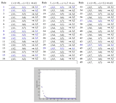
[image:6.595.101.500.378.733.2]

Figure 1. (a) Distribution of sensitivity of input variables, (b) Distribution of singular values of sensitivity matrix We apply the singular value decomposition method in section 4 to get optimal fuzzy relations. The singular values of firing strength matrix are shown in Figure 2. After we take the r most important fuzzy relations, we get ten fuzzy relations that are the optimal number of fuzzy relations. The positions of the ten most important fuzzy relations are known as 1, 2, 8, 9, 10, 15, 17, 29, 37, 44 (blue colored rules in Table 1). The resulted fuzzy relations are used to design fuzzy time series forecasting model (10) or (11).

Table 1. Fuzzy relation groups for interest rate of BIC using generalized Wang’s method Rule (x t( −8),x t(−1)) →x t( ) Rule (x t( −8),x t(−1)) →x t( ) Rule (x t( −8),x t( −1))→x t( )

1 (A1, A1) →A1 17 (A3, A3) →A2 33 (A5, A5) →A1

2 (A1, A2) →A2 18 (A3, A4) →A2 34 (A5, A6) →A2

3 (A1, A3) →A2 19 (A3, A5) →A2 35 (A5, A7) →A2 4 (A1, A4) →A3 20 (A3, A6) →A2 36 (A6, A1) →A2 5 (A1, A5) →A3 21 (A3, A7) →A2 37 (A6, A2) →A2

6 (A1, A6) →A3 22 (A4, A1) →A1 38 (A6, A3) →A2 7 (A1, A7) →A3 23 (A4, A2) →A1 39 (A6, A4) →A2

8 (A2, A1) →A1 24 (A4, A3) →A2 40 (A6, A5) →A2

9 (A2, A2) →A2 25 (A4, A4) →A2 41 (A6, A6) →A2

10 (A2, A3) →A3 26 (A4, A5) →A2 42 (A6, A7) →A2

15 (A3, A1) →A1 31 (A5, A3) →A1 47 (A7, A5) →A2

16 (A3, A2) →A2 32 (A5, A4) →A1 48 (A7, A6) →A2 49 (A7, A7) →A2

(7)

[image:7.595.145.451.263.384.2]

Based on the Table 2, the average forecasting errors of interest rate of BIC using the proposed method and the generalized Wang’s method are 1.8787%, 3.7750% respectively. So we can conclude that forecasting interest rate of BIC using the proposed method results more accuracy than that using the generalized Wang’s method.

Table 2. Comparison of average forecasting errors of interest rate of BIC from the different methods Method Number of

fuzzy relations

MSE of training data

MSE of testing data

Average forecasting errors (%)

Proposed method 10 0.85014 0.14180 1.8787

Generalized Wang’s method 49 1.15250 0.38679 3.7750

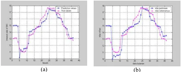
The comparison of prediction and true values of interest rate of BIC using the generalized Wang’s method and the proposed method is shown in Figure 3.

(a) (b)

Figure 3. Prediction and true values of interest rate of BIC using: (a) proposed method, (b) generalized Wang’s method

6. Conclusions

In this paper, we have presented a method to select input variables and reduce fuzzy relations of fuzzy time series model based on the training data. The method is used to get significant input variables and optimal number of fuzzy relations. We applied the proposed method to forecast the interest rate of BIC. The result is that forecasting interest rate of BIC using the proposed method has a higher accuracy than that using generalized Wang’s method. The precision of forecasting depends also on determining number of fuzzy sets and parameter of fuzzy sets. In the future works, we will construct a procedure to determine the optimal fuzzy sets to improve prediction accuracy.

References

[1] Abadi, A.M., Subanar, Widodo, and Saleh, S.(2007). Forecasting interest rate of Bank Indonesia certificate based on univariate fuzzy time series. International Conference on Mathematics and Its applications SEAMS, Gadjah Mada University, Yogyakarta.

[2] Abadi, A.M., Subanar, Widodo, and Saleh, S. (2008a). Constructing complete fuzzy rules of fuzzy model using singular value decomposition. Proceeding of International Conference on Mathematics, Statistics and Applications (ICMSA), Syiah Kuala University, Banda Aceh.

[3] Abadi, A.M., Subanar, Widodo, and Saleh, S. (2008b). Designing fuzzy time series model and its application to forecasting inflation rate. 7Th World Congress in Probability and Statistics, National University of Singapore, Singapore.

[4] Abadi, A.M., Subanar, Widodo, and Saleh, S. (2008c). A new method for generating fuzzy rule from training data and its application in financial problems. The Proceedings of The 3rd International Conference on Mathematics and Statistics (ICoMS-3), Institut Pertanian Bogor, Bogor.

[5] Abadi, A.M., Subanar, Widodo, and Saleh, S. (2009). Designing fuzzy time series model using generalized Wang’s method and its application to forecasting interest rate of Bank Indonesia certificate. Proceedings of The First International Seminar on Science and Technology, Islamic University of Indonesia, Yogyakarta.

(8)

[7] Chen, S.M.. (2002). Forecasting enrollments based on high-order fuzzy time series. Cybernetics and Systems Journal, 33, pp. 1-16.

[8] Chen, S.M., and Hsu, C.C. (2004). A new method to forecasting enrollments using fuzzy time series. International Journal of Applied Sciences and Engineering, 2(3), pp. 234-244.

[9] Golub, G.H., Klema, V. and Stewart, G.W. (1976). Rank degeneracy and least squares problems, Tech Rep TR-456, Dept. Comput. Sci., Univ. Maryland, Colellege Park.

[10] Huarng, K. (2001). Heuristic models of fuzzy time series for forecasting. Fuzzy Sets and Systems, 123, pp. 369-386.

[11] Hwang, J.R., Chen, S.M., and Lee, C.H. (1998). Handling forecasting problems using fuzzy time series. Fuzzy Sets and Systems, 100, pp.217-228.

[12] Saez, D., and Cipriano, A. (2001). A new method for structure identification of fuzzy models and its application to a combined cycle power plant. Engineering Intelligent Systems, 2, pp. 101-107.

[13] Sah, M., and Degtiarev, K.Y. (2004). Forecasting enrollments model Based on first-order fuzzy time series. Transaction on Engineering, Computing and Technology VI, Enformatika VI, pp. 375-378.

[14] Song, Q., and Chissom, B.S. (1993a). Forecasting enrollments with fuzzy time series, Part I. Fuzzy Sets and Systems, 54, pp. 1-9.

[15] Song, Q., and Chissom, B.S. (1993b). Fuzzy time series and its models. Fuzzy Sets and Systems, 54, pp. 269-277.

[16] Song, Q., and Chissom, B.S. (1994). Forecasting enrollments with fuzzy time series, Part II. Fuzzy Sets and Systems, 62, pp. 1-8.