Conference paper

COMBINED MULTI-VIEW MATCHING ALGORITHM WITH LONG-STRIPS OF

SATELLITE IMAGERY FROM DIFFERENT ORBITS

Jinxin Xiong a, _{*, Yongjun Zhang} a

a

_{School of Remote Sensing and Information Engineering; Wuhan University, Wuhan 430049, China –}

einbetter1995@hotmail.com

Commission Ⅲ, WG Ⅲ/1

KEY WORDS: Matching, Satellite Imagery, Long Strips, Multiple Orbits, Chinese Mapping Satellite-I

ABSTRACT:

Existing matching algorithms aim to match conjugate points among overlapping satellite scenes acquired from the same orbit and can generally achieve good matching performance. Unfortunately, no algorithm can avoid the difficulty of simultaneously processing the data sets of long-strip imagery acquired from different orbits. In this paper, the combined matching algorithm we propose introduces the LBP/C operator, which, when combined with existing feature detectors for the first time, can make possible the extraction of more stable interest points and candidates. At the same time, based on the typical characteristics of Chinese satellite imagery, we improved the filter method and achieved an effective combination of several image matching algorithms. A comparison among several kinds of matching transfer modes was presented; and to evaluate this algorithm, Chinese Mapping Satellite-I data are used as the reference data.

1. INTRODUCTION

Image matching was a key technology related to many problems in computer vision and photogrammetry, including object recognition, motion tracking, digital surface model (DSM) generation, etc. (Lowe, 2004). In the past 20 years, research related to processing satellite imagery has become a key focus. Due to the position and attitude information under fixed sampling intervals, the current matching algorithms are focused on area-based algorithms, especially the approximate epipolar geometric constraints (Heipke, 1996). These existing algorithms can achieve satisfactory matching results in the case of overlapping scenes acquired from the same orbit, but they cannot solve the following problems: 1) how to match with multiple long-strip satellite imagery simultaneously 2) how to eliminate the radiometric and geometric differences between adjacent orbits and achieve high-accuracy results. Moreover, the typical characteristics of imagery acquired from Chinese satellites (e.g., ambiguity in smooth areas, low direct geo-referencing accuracy, and obvious differences in contrast) bring more challenges to image matching. Consequently, finding solutions for the above-mentioned problems in photogrammetry was an urgent issue.

In this study, we developed a practical matching algorithm based on the approaches in the literature. First, we divided the reference strip of imagery in each orbit into independently overlapping image patches; then, each patch was filtered to enhance the existing texture patterns and improve the noise-signal ratio (Baltsavias, 1991). After the generation of image pyramids, we combined the Harris-Z detector (Bellavia, 2008) with the LBP/C operator (Timo, 2002) to extract stable interest points. At the same time, the Förstner interest operator (Förstner, 1986) was used to refine these interest points. Then, through the global digital elevation model (Global DEM), the approximate geography scope covered by each image patch was computed. Moreover, the Geometrically Constrained Cross-Correlation (GC3_{) algorithm (Zhang, 2005 and 2006) was} extended to match multiple long-strip imagery; and finally,

several strategies were proposed to detect and eliminate the mismatches. By comparing the results of several matching transfer modes, we determined the optimal manner in which to optimize the matching speed and reduce the number of mismatches.

In the second part, the new matching algorithm is described in detail, and the validity of the proposed matching algorithm is verified with Chinese Mapping Satellite-I data.

2. METHODOLOGY

In this paper, the proposed algorithm includes four parts: 1) Image Pre-Processing; 2) Image Matching Procedure; 3) Mismatch Detection and Elimination.

2.1 Image Pre-Processing

Image pre-processing method includes two parts: 1) Modified Wallis Filter; 2) Interest Points and Candidates Detection and Extraction

2.1.1 Modified Wallis Filter

Compared with aerial imagery and close-range imagery, the characteristics of satellite imagery generally include the following: 1) low spatial resolution, 2) unsymmetrical contrast of light and shade, 3) fuzzy texture structure. These factors seriously affect the reliability of feature extraction and image matching.

To solve these problems mentioned above, the Wallis filter is introduced. It can force the mean and contrast of an image to fit some given values effectively. Baltsavias (1991) used this filter to enhance the image texture pattern and eliminate radiometric difference. The general form of the Wallis filter is given by:

g

w

( , )

x y



g

( , )

x y r r

1



0 ₍₁₎

Where

1 f g f

0 f 1 g

= c / (c + / c)

= b +(1- b - )

r

s

s s

r

m

r m

₍₂₎

In Equation 1,

g

w( , )x y and

g

( , )x y are the filtered and original image respectively, r0 and

r

1 _{are the additive and} multiplicative parameters,

m

g _and

s

g _{are the mean and} standard deviation of the original image,

m

f _and

s

f _{are the}

target values for the mean and standard deviation,

c

was the contrast expansion constant, and b was the brightness forcing constant.

However, the existing Wallis filter has some problems: 1) the edges of roofs tend to expand, which causes deviations from their geometrical position; and 2) the image noise is partially enhanced, which hurts the positioning accuracy of the features extracted and has a detrimental effect on image matching. We found that the additive parameter r0 causes the above

problems. Owing to its restrictions on the gray level, unreasonable selection of

r

0 _{causes the excessive loss of gray}

information for the following reasons. First, r0 is mainly

dependent on parameter b ; secondly, the multiplicative parameter

r

1 _{can change image contrast, whose value is} dependent on parameter

c

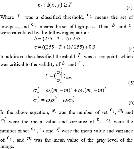
; and lastly, the high texture fidelity and enhance image contrast must be kept under the filter’s capacity. In this study, we used the following method to improve the Wallis filter.

A highly adaptive parameter determination strategy: In the case of an image f(x,y), we classified all pixels of this image into

were calculated by the following equation:

In addition, the classified threshold

T

was a key point, which was critical to the validity of b and

c

:

2.1.2 Interest Points and Candidates Detection and Extraction:

Strong relationships exist between the probability of the correct matching and the texture information content. Although detailed rules differ by surface variation, it has been shown that a successful rate of matching increases the probability of enriched texture information.

As a powerful tool for texture classification, the Local Binary Pattern (LBP) operator was an excellent measure of the spatial structure of local image texture. Ojala (2002) developed the LBP operator, which allows for detecting “uniform” patterns in circular neighborhoods of any quantization of the angular space and spatial resolution. Moreover, he enhanced the performance of the LBP operator through combining it with a rotation invariant local contrast (LC) measure that characterizes the contrast of local image texture.

In the case of an image, texture T was the joint distribution of the gray levels:

T



t

( , ,...,

g g

c 0

g

P1

)

₍₇₎ Where P (P>1) was the number of neighboring pixels, gray value gcwas the center pixel of the local neighborhood, and

P

g _{was the neighboring pixel on a circle of radius R, as shown} in Fig. 2. The coordinates of gP were calculated using

Figure 1: Circularly symmetric neighbor sets for different (P, R)(Ojala, 2002)

In fact, without losing information, the signed differences between the gray value of

g

c _and

g

P _{(P=0,…P-1) were not} affected by variation in the mean luminance. Hence, the joint difference distribution was invariant against the grayscale shifts. By considering the signs of the differences, instead of

transformed Equation 9 into a unique LBP value. In this study, we set (P=12,R=1.5): “uniform” and proposed the following operator for grayscale and rotation invariant texture description instead ofLBPP R, _:

1

The LBPP Rriu,2 _{operator was a grayscale invariant measure. It} was an excellent measure of the spatial pattern, but it discarded contrast. So a rotation invariant measure was introduced to characterize the contrast of the local image texture:

1

2 ,

0

1P _{( )}

P R p

p

LC g

P













(14) Where

1

p=0

1 = P g_p

P







,

P R

LC _{was an invariant against shifts in grayscale. Since} 2

,

riu P R

LBP _and LCP R, _{are complementary, their joint}

distribution LBPP Rriu, 2/LCP R, _{, was expected to be a very} powerful rotation invariant measure of local image texture. When we compared feature detectors, Harris-Z was found to be more suitable to detect the interest points for large data sets of satellite imagery in our study. We also introduced the Förstner detector at this point and the surface fitting approach to get sub-pixel positioning. In this study, we combined Harris-Z with LBP/C to detect the stable interest points and candidates that optimize the validity of matching, which included the following five steps:

1) To ensure uniform distribution of the interest points, we used the grid of the feature extraction as a region unit, and a fixed number of features were extracted in each unit independently.

2) The interest strengths and LBP/C values in a region unit were calculated by the Harris-Z detector and the LBP/C operator.

3) Some points were saved when their LBP/C values were in a certain range. Then, we chose the point with the local maximum interest strength as the interest point that corresponded to the region unit. As a candidate, we chose the point with the maximum interest strength without consideration for its LBP/C value.

4) We used the Förstner detector and the surface fitting approach to obtain the sub-pixel positioning of the interest point and candidate.

5) Once the interest point failed to match or the accuracy of this match was low, the candidate was matched rather than the interest point; and the match with the higher accuracy was saved.

2.2 Image Matching Procedure

Due to linear pushbroom imaging mode, we can calculate the exterior orientation corresponding to every scanline through lagrangian interpolation. Thereby, in this paper, the proposed matching algorithm is based on the geometrically constrained cross-correlation. The algorithm includes the following several studies:

2.2.1 Automatic Computation for Approximate Elevation Range and Elevation Step through Global DEM

According to the position and attitude information of the scan lines, we use a hypothesis height to the frontal-project four corners of the corresponding reference image patch onto the ground. The approximate geography scope covered by the image patch was determined, and the maximum elevation Hmax

and the minimum elevation Hmin _{are achieved through} retrieval from Global DEM.

Then, we frontal-projected an interest point extracted onto the ground using

H

max _and

H

min_{, and back-projected these} object space points onto all of the search strips. The corresponding image coordinates (ximax_, ymaxi _{), (}

x

mini _,ymini )

then could be determined, where i was the index of the different search strips. After that, we calculated the elevation step Hpitchi _{with the following equation:}

(

) /

i i

H

_pitch



H

_max



H

_min

Length

(15)

Where

(

) (

2

)

2

i

i i i i

Length



x

_max



x

_min



y

_max



y

_{min (16)}

It was an iterative process: once Hpitchi _{was an invalid value,} we had to repeat the above procedure using another interest point.

2.2.2 Geometric and Radiometric Distortion Procedure There were geometric and radiometric distortions in the case of strips acquired from different camera lenses. When the correlation window is defined in the reference image, this kind of distortion leads to an irregular and discontinuous shape of the corresponding window in the search images, which cannot be matched in a straightforward manner.

Gruen and Baltsavias (1985) extended the LSM method, which compensates this distortion and relaxes the strict geometric and radiometric assumption for normal cross-correlation methods. So, we introduced this method to eliminate the window warping:

1) In the reference image, we defined a correlated window Л and a search window Г in which an interest point or candidate was central, then the corresponding pixel coordinates of the four corners and the center of Г were achieved by projection in the search image, which formed an irregular polygon Г’, as shown in Fig. 2. Accordingly, we calculated the parameters of the affine geometric transformation and linear radiometric transformation between these images.

x

2



a a x a y

0



1



2 ₍₁₇₎

y

2

 

b b x b y

0 1



2 ₍₁₈₎

g x y

( , )



h h g x y

0



1 2

( , )

2 2 ₍₁₉₎

Where a0, a1, a2, b0 , b1, b2 were the parameters of the affine geometric transformation;

h

0_,

h

1 _{were the parameters}

of the linear radiometric transformation.

2) Through Equations 17 and 18, the relationship of each pixel between Г and Г’ was determined. The gray values in Г’ were interpolated by bilinear interpolation, and these gray values, recalculated by Equation 19, were assigned to the corresponding pixel in Г.

' 

G lo b a l D E M

R e fe r e n c e Im a g e P ( X ,Y ) p (x ,y )

 '

0 1 2 '

0 1 2 0 12 2 2 ( , ) ( , ) x a a x a y y b b x b y g x y h h g x y

       

S e a r c h I m a g e

Figure 2. The principle of the affine geometric transformation and linear radiometric transformation between the reference

image and search image

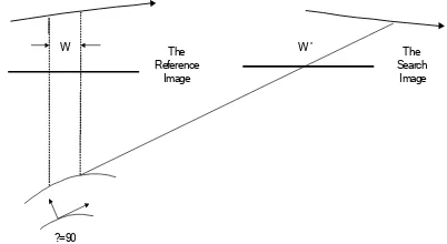
3) Once the angle θ was greater than 90 degrees on the very steep terrain surface, as shown in Fig. 3, W’ became zero and mafe the procedure impossible. In this case, we found that when we iteratively computed the parameters of the transformation, the convergent speed was slow, and even the computation was divergent. So once the threshold of iteration times was crossed, we considered θ≥90 and excluded it.

W _The W ’

Reference Image

The Search Image

?=90

Figure 3. Image selection or exclusion based on the terrain slope and the sensor geometry. The size of the corresponding correlation window in the search image depends on the angle θ

between the normal vector of the local object surface and the corresponding imaging ray.

4) The correlation window and search window are both square as shown in Fig. 4. Therefore, we could do a straightforward match and reduce the computational cost.

2.2.3 Extended Geometrically Constrained Cross-Correlation Strategy

Based on the area-based matching techniques, Zhang developed GC3 _{(Geometrically Con-strained Cross-Correlation)} algorithm. With the GC3 _{matching procedure, multiple images} can be matched simultaneously and the epipolar constraint is integrated implicitly. As a similarity measure, SNCC (Sum of Normalized Cross-Correlation) greatly decreases mismatches caused by approximate texture distinction and occlusion problem. However, this algorithm causes high computational costs in determining the correct height value and has redundance for its quality measuring procedure. Basically we extended this algorithm and save the computational costs: 1) For each reference image patch, the approximate elevation range and elevation step can be determined. After pre-processing the reference image patch, for each interest point or candidate, the corresponding approximate epipolar lines in the search strips can be further determined.

2) According to the position of approxi- mate epipolar lines, we define the search image patches, and pre-process them. 3) Based on geometric and radiometric distortion procedure, we calculate the parameters of affine geometric transformation and linear radiometric transformation between the defined windows.

4) We combine a coarse-to-fine hierarchical approach with the efficient implementation of the epipolar geometry to match each point on the approximate epipolar lines. Once normalized cross-correlation coefficient in the certain level of pyramids is lower than threshold, we repeat the above procedures with different elevation in the certain range.

5) Until accomplishing the matching procedure, we compute the SNCC of all matching candidates.

6) Determine the sites of local maxima of the SNCC function and fit a smooth quadratic function for each local maximum with a local neighborhood of that maximum value.

7) If the second SNCC peak is less than half or one third of that of the first SNCC peak, the peak that have the largest SNCC value should represent the correct match. If not, we match inversely and if the difference between the two matches is less than 1.5 pixels in image space, the candidate should be the correct match.

8) Repeat 1)-7), until all interest points and candidate are matched.

2.3 Mismatches Detection and Elimination

After finishing the image matching procedure, there are inevitably some blunders that do not conform to the geometrical relationship in an object space, which we call mismatches. To maintain the matching accuracy, we must eliminate mismatches as accurately as possible. Thus, we classify all of the matches into two types, interior matches and adjacent matches. In this section, we present two strategies to eliminate mismatches

2.3.1 Mismatches Elimination Strategy within Orbit: In this study, we introduce the multi-rays forward intersection principle to eliminate mismatches and realize the object fusion for the matching results. The implementation strategy was as follows:

1) If an interest point or candidate finds multiple correspondences on the search strips, we assume that the exterior orientation elements corresponding to each image are known. We take the 3D coordinates of all matches in the object space as unknown; and based on the collinearity equations, we then list the error equations:

V

x



a dX a dY a dZ l

11



12



13



x ₍₂₀₎

V

y



a dX a dY a dZ l

21



22



23



y ₍₂₁₎

Where a11_,

a

12_,a13_,a21,a22_,

a

23 _{are the parameters related to}

the line elements of the exterior orientation; lx _, ly _are

differences between observations and approximations.

2) If the number of the correspondences is n, we can list (2n+2) error equations. To solve the iterative computation for unknown numbers, the least square adjustment was introduced. In the iterative procedure, we set the weights of each observation of the image points through a hypothesis test of the posterior variance component. If there are grosses in the candidates, the observation weights of the candidates become smaller and smaller until 0 was reached, which makes no sense in the adjustment process in order to eliminate the effect of a false match on the calculation of effectiveness.

3) After iterative convergence was achieved or the iterative times exceed the limited value, the root mean square (RMS) value was calculated. Once the RMS exceeds the given threshold, the corresponding matches are eliminated.

2.3.2 Mismatches Elimination Strategy between Adjacent Orbits

Once the position and attitude parameters acquired from different orbits exhibited obvious system shift, the matches between the adjacent orbits could not be intersected together in the object space. If we used the above strategy, we would face the problem of iterative computation convergence. Therefore,

we introduced an Object Space Shift (OSS) strategy to eliminate mismatches between the adjacent orbits:

1) The correspondences P1, P2, …, Pn between the adjacent orbits were intersected within each orbit, and the shift of each point in the object space were calculated ( X△ 1, Y△ 1, Z△ 1), ( X△ 2, Y△ 2, Z△ 2), …, ( X△ n, Y△ n, Z△ n). Then, the mean shift Ax_, Ay_, Az _{were calculated in Equation 22:}

1 2 3 1 2 3 1 2 3

( ) /

( ) /

( ) /

x n

y n

z n

A X X X X n

A Y Y Y Y n

A Z Z Z Z n

       

       

        ₍₂₂₎

The mean square values in each direction

m

x_,

m

y_,

m

z _were

calculated in Equation 23, and the RMS merror _{between the} adjacent orbits were calculated in Equation 24.

2 2 2 2

1 2 3

2 2 2 2

1 2 3

2 2 2 2

1 2 3

(( ) ( ) ( ) ( ) )/ (( ) ( ) ( ) ( ) )/ (( ) ( ) ( ) ( ) )/

x x x x n x

y y y y n y

z z z z n z

m X A X A X A X A n

m Y A Y A Y A Y A n

m Z A Z A Z A Z A n

           

           

            ₍₂₃₎

m

error



(

m m m m m m

x



x



y



y



z



z

)

₍₂₄₎

2) Once the shift Ti was more than triple merror_{, we deemed} this correspondence as a mismatch.

2 2 2

(

) (

) (

)

i i x i y i z

T

  

X A

  

Y A

  

Z A

Ti 3 merror: MisMatch ₍₂₅₎

3 orrect Match

i error

T m ： C

3. EXPERIMENTS AND ANALYSIS

3.1 Test Data Description

Figure 4 shows the real data for experiment, which consists of two long strips of imagery acquired by Chinese Mapping Satellite. These data are imaged on October, 2010, which covers Harbin in China, the coverage area is about 25000km2_. The satellite sensor works in pushbroom mode, and the stereo module consists of three lenses with one CCD line scanner for each, which provide a forward-, a nadir- and a backward-looking view. The degree of overlapping within orbit is about 98%, and the degree between adjacent orbits is about 10%. The parameters of CCD line sensors are shown in table 1.

Table 1. Camera parametres of the three linear array sensor for Chinese Mapping Satellite

Parameter Forward-View Nadir-View Backward-View

Focal Length (mm) 717 650 717

GSD (m) 5.0 5.0 5.0

Intersection Angle

(deg) 25.0 0.0 -25.0

Pixel Size (mm) 0.0065 0.0065 0.0065

Scan Line Width

(pixel) 12000 12000 12000

Length of Strip

(pixel) 142862 238100 142862

Geographical Scope

(km2₎ 42858.6 71430.0 42858.6

Data Volume (GB) 4.46 7.31 4.46

Base-Height Ratio 0.9323

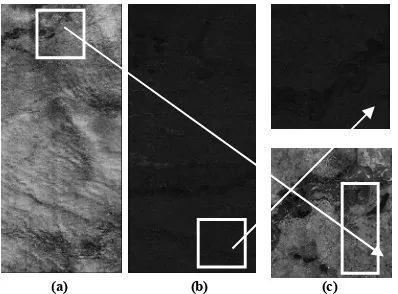
Figure 4. The Nadir-looking strips in the adjacent orbits: (a) The nadir-looking strip acquired from the first orbit; (b) The nadir-looking strip acquired from the second orbit; (c) The enlarged drawing of the overlapping area between the two

strips

For testing and verifying the accuracy and reliability of the proposed algorithm, the geographical region covered by the test data includes not only farms and forests which have strong texture repeatability, but also residential quarters, mountain countries and smoothly open areas which are known as difficult terrain for matching. In addition, in order to analyze the matching accuracy quantitatively, the test data includes 33 planar control points and 15 elevation control points. After finishing the matching procedure, the ground control points are measured interactively on the test imagery, and then the bundle block adjustment is performed with matching points and control points.

3.2 Image Matching Testing

In order to improve the performance of the proposed matching algorithm, we compare different parameters in two ways: the number of pyramid levels and the size of the relative window at the top level.

(a)

(b)

Figure 5. The successful rate of matching using the number of pyramid levels and the size of the relative window at the top level: (a) the effect of different number of pyramid levels; (b) the effect of different size of relative window at top level

(a) (b) (c)

Figure 5 shows the results in which the number of pyramid levels and the size of the relative window at the top level are varied. In graph (a), when the number is 3, the successful rate of matching is the highest toward the different terrain types. In graph (b), it is poor at the successful rate when the relative windows is set 7×7 pixels, but the results are not improved

till 13×13 pixels. After that, a larger size of relative window

can actually hurt the matching. Although the successful rate for 13×13 is a little lower than 11×11 and 9×9 on mountain countries and farms respectively, the overall successful rate is optimum. Therefore, through this experiment, we generate three pyramid levels and set the size of the relative window R×R as 13×13. Moreover, the relative window is shrank to (R-2)×(R-2) level to level, and the corresponding search window is (2×R-1)*(2×R-1). The matching results are listed in table 3.

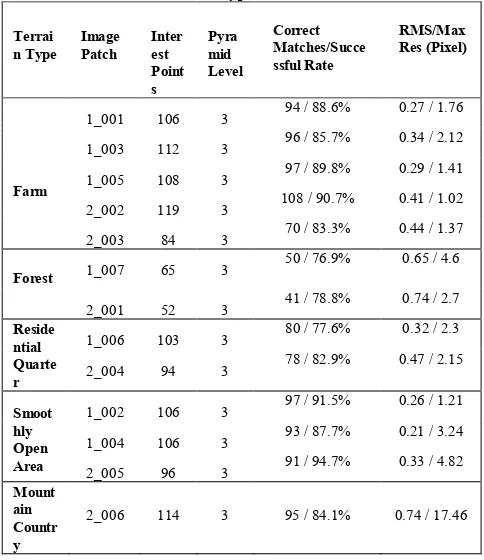
Table 3. Matching accuracy quantitative evaluation for different types of terrain

Terrai

n Type Image Patch Interest

Point s

Pyra mid Level

Correct Matches/Succe ssful Rate

RMS/Max Res (Pixel)

1_001 106 3 94 / 88.6% 0.27 / 1.76 1_003 112 3 96 / 85.7% 0.34 / 2.12 1_005 108 3 97 / 89.8% 0.29 / 1.41 2_002 119 3 108 / 90.7% 0.41 / 1.02

Farm

2_003 84 3 70 / 83.3% 0.44 / 1.37 1_007 65 3 50 / 76.9% 0.65 / 4.6

Forest

2_001 52 3 41 / 78.8% 0.74 / 2.7 1_006 103 3 80 / 77.6% 0.32 / 2.3

Reside ntial Quarte

r 2_004 94 3

78 / 82.9% 0.47 / 2.15

1_002 106 3 97 / 91.5% 0.26 / 1.21 1_004 106 3 93 / 87.7% 0.21 / 3.24

Smoot hly Open

Area _{2_005 96 3} 91 / 94.7% 0.33 / 4.82

Mount ain Countr y

2_006 114 3 95 / 84.1% 0.74 / 17.46

Table 3 illustrates the statistics of image matching for the test date on five types of terrain, through analysis for the matching results, we can see that:

1) For farms and forests which have strong texture repeatability, the range of the successful rate of matching is from 76.9% to 90.7%. Especially in areas covered by farms, the RMS error is within 0.5 pixel, which means that the proposed algorithm can avoid mismatching problem caused by texture repeatability.

2) For residential quarter and smoothly open areas, there are a few false matches, but most of matches are fine, the range of the successful rate is from 77.6% to 94.7%, the range of RMS error is from 0.21 to 0.47 pixel. Thus, the matching result is satisfactory.

3) For mountain countries, because of the rise or descend on terrain greatly, there are some obviously false matches, which greatly affect the precision of matching. But the RMS error is

still 0.74 pixel, which proves that the matching algorithm can be applied to this terrain.

4. CONCLUSION

In this study, we develop a practical algorithm for matching with large data sets of long-strips of satellite imagery. Through some experiments using real data set from Chinese Mapping Satellite, the proposed algorithm are proved to be valid, and the satisfactory accuracy is achieved under fully automatic computation.

At the present stage, the proposed methods mostly focus on multi-view matching with long strips of satellite imagery acquired from different orbits. In the futhre, we will keep on this research and realize the matching algorithm that support various satellite sensors, even various imaging modes.

REFERENCES

DAVID, G. LOWE. 2004. Distinctive Image Features from Scale-Invariant Keypoints. International Journal of Computer Vision, Vol. 60, No. 2, pp. 91-110

Heipke, C. 1996. Overview of image matching techniques. In Proceedings of OEEPE Workshop on the Application of Digital Photogrammetric Workstations, Lausanne, Switzerland, Part III

Baltsavias, E.P. 1991. Multiphoto geometrically constrained matching. Ph.D. dissertation, Institute of Geodesy and Photogrammetry, ETH Zurich, Report No. 49.

F.Bellavia, D.Tegolo, C.Valenti. 2008. A non-parametric scale-based corner detector. Pattern Recognition (ICPR), 19th International Conference, pp, 1-4

Timo, Ojala and Matti, Pietikäinen. 2002. Multisolution Gray-Scale and Rotation Invariant Texture Classification with Local Binary Patterns. IEEE Transaction on Pattern Analysis and Machine Intelligence, Vol. 7, No. 24, pp. 971-987

Foerstner, W. 1986. A Feature Based Correspondence Algorithm for Image Matching. Proceedings of the Symposium from Analytical to Digital, August 19-22, Rovaniemi, Finland, pp. 150-166.

Zhang, Li. 2005. Auto Digital Surface Model (DSM) Generation from Linear Array Images. Zurich: Ph. D. Dissertation, ETH Zurich, Switzerland

Zhang, L., Gruen, A. 2004. Automatic DSM Generation from Linear Array Imagery Data. IAPRS, Vol. 35, Part B3, pp. 128-133

Q. Zhu., B. Wu., N. Wan. 2006. An interest point detect method to stereo images with good repeatability and information content. Acta Electron. Sin, Vol. 34, No. 2, pp. 205–209

Gruen, A and Baltsavias, E. P. 1985. Adaptive Least Squares Correlation with Geometrical Constraints. SPIE, Vol. 595, pp. 72-82

Gruen, A. and Baltsavias, E. P. 1988. Geometrically Constrained Multiphoto Matching. PE&RS, Vol. 54, No. 5, pp. 633-641