SEMI-SUPERVISED MARGINAL FISHER ANALYSIS FOR HYPERSPECTRAL IMAGE
CLASSIFICATION
Hong Huang, Jiamin Liu and Yinsong Pan
Key Lab. on Opto-electronic Technique and systems, Ministry of Education Chongqing University, Chongqing, China
Commission III, ICWG III/VII
KEY WORDS:Hyperspectral image classification, dimensionality reduction, semi-supervised learning, manifold learning, marginal Fisher analysis
ABSTRACT:
The problem of learning with both labeled and unlabeled examples arises frequently in Hyperspectral image (HSI) classification. While marginal Fisher analysis is a supervised method, which cannot be directly applied for Semi-supervised classification. In this paper, we proposed a novel method, called semi-supervised marginal Fisher analysis (SSMFA), to process HSI of natural scenes, which uses a combination of semi-supervised learning and manifold learning. In SSMFA, a new difference-based optimization objective function with unlabeled samples has been designed. SSMFA preserves the manifold structure of labeled and unlabeled samples in addition to separating labeled samples in different classes from each other. The semi-supervised method has an analytic form of the globally optimal solution, and it can be computed based on eigen decomposition. Classification experiments with a challenging HSI task demonstrate that this method outperforms current state-of-the-art HSI-classification methods.
1 INTRODUCTION
With the development of the remote-sensing imaging technology and hyperspectral sensors, the use of hyperspectral image (HSI) is becoming more and more widespread, such as target detection and land cover investigation. Due to the dense sampling of spec-tral signatures of land covers, HSI has a better potential discrimi-nation among similar ground cover classes than traditional multi-spectral scanners (Li et al., 2011, Guyon and Elisseeff, 2003, D. Tuia et al., 2009). However, classification of HSI still faces some challenges. One major challenge is that the number of training samples is typically limited compared with the dimensionality of the data (Huang er al., 2009). This procedure usually results in a loss of accuracy as the data dimensionality increases, which is called the curse of dimensionality (Chen and Zhang, 2011, Kaya et al., 2011). Therefore, the most important and urgent issue is how to reduce the number of those bands largely, but without loss of information (Yang et al., 2011, Paskaleva et al., 2008).
The goal of dimensionality reduction is to reduce complexity of input data while some desired intrinsic information of the data is preserved. Techniques for representing the data in a low-dimen-sional space can be subdivided into two groups (Huang et al., 2011, Huang et al., 2011): (1) linear subspace algorithms; (2) manifold learning based nonlinear algorithms. Principal com-ponent analysis (PCA) and Linear discriminant analysis (LDA) are the most popular subspace methods among all dimension-ality reduction algorithms, which seek linear subspaces to pre-serve the desired structure of the data in the original Euclidean space. In recent years, many researchers have considered that the real-world data may lie on or close to a lower dimensional man-ifold. The representative of such methods include locally linear embedding (LLE) (Roweis and Saul, 2000), isometric mapping (Isomap) (Tenenbaum et al., 2000), and Laplacian eigenmaps (Belkin and Niyogi, 2003), etc. However, these methods are de-fined only on training data, and the issue of how to map new test data remains difficult. Therefore, they cannot be applied directly to problems.
Recently, some algorithms resolve this difficulty by finding a
mapping on the whole data space, rather than on training data. Locality Preserving Projection (LPP) (He et al., 2005) and neigh-borhood preserving embedding (NPE) (He et al., 2005) are de-fined everywhere in the ambient space rather than just on the training data set. Then, LPP and NPE outperform LLE and LE in locating and explaining new test data in the feature subspace. However, the two algorithms, like Isomap, LLE and LE, do not make use of the class label information, which is much avail-able for classification tasks. Cai et al. (Cai et al., 2007) pre-sented a Locality Sensitive Discriminant Analysis (LSDA) algo-rithm to find a projection which maximizes the margin between data points from different classes at each local area. Another dis-criminant analysis method should be mentioned here, which is called marginal Fisher analysis(MFA) (Yan et al., 2007). MFA provides a proper way to overcome the limitations of LDA, and a new criterion for MFA is designed to obtain an optimal trans-formation by characterizing the intra-class compactness and the inter-class separability.
Most of the existing discriminant methods are fully supervised, which can perform well when label information is sufficient. How-ever, in the real world, the labeled examples are often very diffi-cult and expensive to obtain. The traditional supervised methods cannot work well when lack of training examples; in contrast, unlabeled examples can be easily obtained(Camps-Valls et al., 2007, Velasco-Forero et al., 2009, D. Tuia et al., 2009). There-fore, in such situations, it can be beneficial to incorporate the in-formation which is contained in unlabeled examples into a learn-ing problem, i.e., semi-supervised learnlearn-ing (SSL) should be ap-plied instead of supervised learning (Song et al., 2008, Zhu and Goldberg, 2009, Zha and Zhang, 2009).
compactness between data points belong to the same class or neighbors.
The remaining of the paper is organized as follows. In Section 2, we first present a brief review of MFA , and discuss the limita-tions of this algorithm. The SSMFA method is introduced in Sec-tion 3. SecSec-tion 4 presents the experimental results on both illus-trative toy examples and several hyperspectral image databases to demonstrate the effectiveness of SSMFA. Finally, we provide some concluding remarks and suggestions for future work in Sec-tion 5.
2 RELATED WORKS
In this section, we provide a brief review of marginal Fisher anal-ysis (MFA) (Yan et al., 2007), which is relevant to our proposed method. We begin with a description of the dimensionality re-duction problem.
2.1 The Dimensionality Reduction Problem
The generic dimensionality reduction problem is as follows. Given ndata pointsX = {x1,x2, . . . ,xn} ∈ ℜm×n sampled from one underlying manifoldM, andℓi ∈ {1, . . . , c}denotes the class label of xi. The goal of dimension reduction is to map (X∈ ℜm)7→(Y∈ ℜd)whered≪mby using the information of examples.
2.2 Marginal Fisher Analysis (MFA)
To overcome this limitation of Linear discriminant analysis (LDA), marginal Fisher analysis (MFA) was proposed by developing a new criterion that characterized the intra-class compactness and the inter-class separability to obtain the optimal transformation.
In order to discover both geometrical and discriminant structure of data points, MFA designs two graphs that characterize the intra-class compactness and inter- class separability, respectively. The intrinsic graphGcillustrates the intra-class point adjacency relationship, and each sample is connected to itsk-nearest neigh-bors that belong to the same class. The penalty graphGp illus-trates the inter-class marginal point adjacency relationship, and the marginal point pairs of different classes are connected.
LetN+ neighbors. Thus, the weight matrixWc of Gc can be defined as follows
Then, the intra-class compactness is defined as the sum of dis-tances between each node and itsk1-nearest neighbors that be-long to the same class:
P
We consider each pair of points (xi,xj) from the different classes, and add an edge betweenxiandxjifxjis one ofxi’sk2-nearest neighbors whose class labels are different from the class label of
xi. LetNk−2(xi) ={x neighbors. The weight matrixWpofGpcan be defined as
Wp,ij=
The interclass separability is characterized by a penalty graph with the term
Then, the Marginal Fisher Criterion is defined as follows:
arg min
V
VTXLcXTV
VTXLpXTV
(5)
The projection directionVthat minimizes the objective function (5) can be obtained by solving the generalized eigenvalue prob-lem:
XLcXTv=λXLpXTv (6)
3 SEMI-SUPERVISED MFA (SSMFA)
In this section, we introduce the SSMFA method, which respects both discriminant and manifold structures in the data. We begin with a description of the semi-supervised dimensionality reduc-tion problem.
3.1 The Semi-supervised Dimensionality Reduction Prob-lem
The generic semi-supervised dimensionality reduction problem is as follows. Givenndata pointsX={xi, x2, . . . , xn} ∈ ℜm sampled from one underlying manifoldM, suppose that the first lpoints are labeled, and the restn−lpoints are unlabeled. Let ℓi ∈ {1, . . . , c}denote the class label ofxi. The goal of semi-supervised dimension reduction is to map(X∈ ℜm) 7→ (Y ∈
ℜd)
whered≪mby using the information of both labeled and unlabeled examples.
3.2 SSMFA
To improve MFA, we consider to exploit the optimal discriminant features from both labeled and unlabeled examples, and it also treats the labeled and unlabeled data differently to construct the objective function for maximizing the inter-class margin while minimizing the intra-class disparity.
We assume that naturally occurring data may be generated by structured systems with possibly much fewer degrees of freedom than what the ambient dimension would suggest. Thus, we con-sider the case when the data lives on or close to a manifoldMof the ambient space. In order to model the local geometrical struc-ture ofM, we first construct a nearest neighbor graphG. For each data pointxi, we find itsknearest neighbors and put an edge be-tweenxiand its neighbors. LetN(xi) ={x1i,x
2
whereσis the local scaling parameter.
The nearest neighbor graphGwith weight matrixAcharacterizes the local geometry of the data manifold. However, this graph fails to discover the discriminant structure in the data. In order to discover both geometrical and discriminant structures of the data manifold, we construct two graphs, that is,between-manifold graphGbandwithin-manifoldgraphGw.
Forbetween-manifoldgraphGb, theith node corresponds to data pointxi. Then, we put an edge between nodesiandjifxiand
xiandxihave different class labels. Forwithin-manifoldgraph Gw, we put an edge between nodesiandjifxiandxihave the same class labels orxiorxjis unlabeled but they are close, i.e.
xiis amongk3nearest neighbors ofxjorxjis amongk3nearest neighbors ofxi. LetNkl3(xi) ={x
1 i,x
2
i, . . . ,xki3}denotes the set of itsk3nearest neighbors inGw.
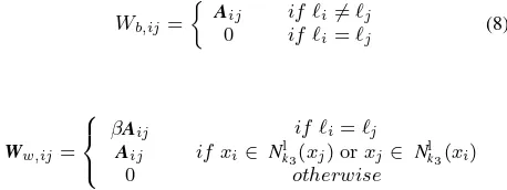
Once the graphsGbandGware constructed, their affinity weight matrices, denoted byWbandWw, respectively, can be defined as
Wb,ij= whereβ >1is a trade-off parameter, which is used to adjust the contribution of labeled and unlabeled data. When two data share the same class label, it is with high confidence that they live on a same manifold. Therefore, the weight value should relatively be large.
The objective of SSMFA is embodied as that it maximizes the sum of distances between margin points and their neighboring points from different classes, and minimizes the sum of distances between data pairs of the same class and each sample inNlto its k3-nearest neighbors. Then, a reasonable criterion for choosing an optimal projection vector is formulated as
arg max
The objective function (10) on thebetween-manifoldgraphGbis simple and natural. IfWb,ij6= 0, a good projection vector should be the one on which those two samples are far away from each other. With some algebraic deduction, (10) can be simplified as
Jb(V) =P
The objective function (11) on thewithin-manifoldgraphGwis to find a optimal projection vector with stronger intra-class/local compactness. Following some algebraic deduction, (11) can be
simplified as
Then, the objective function (10) and (11) can be reduced to the following:
maxVTXLbXTV minVTXLwXTV
(14)
From the linearization of the graph embedding framework, we have the Semi-supervised Marginal Fisher Criterion
V∗= arg max
The optimal projection vectorvthat maximizes (15) is general-ized eigenvectors corresponding to thedlargest eigenvalues in
XLbXTv=λXLwXTv (16)
Let the column vectorv1,v2, . . . ,vdbe the solutions of (16) or-dered according to their eigenvaluesλ1≤λ2≤. . .≤λd. Thus, the projection vector is given as follows:
V∗= [v1,v2, . . . ,vd] (17)
4 EXPERIMENTS AND DISCUSSION
In this section, we compare SSMFA with the several represen-tative dimensionality reduction algorithms on synthetic data and two well-known hyperspectral image databases.
4.1 Experiments on synthetic data
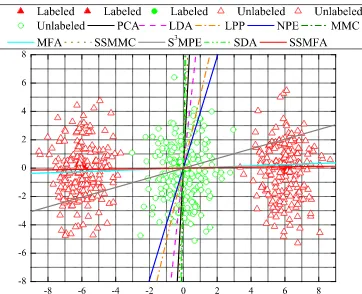
To illustrate the dimensionality reduction capability of the pro-posed SSMFA algorithm, we present dimensionality reduction examples of PCA, LDA, LPP (He et al., 2005), NPE (He et al., 2005), MMC (Li et al., 2006), MFA (Yan et al., 2007), SSMMC (Song et al., 2008),S3
MPE (Song et al., 2008), SDA (Cai et al., 2007) and SSMFA, where two-class synthetic data samples are embedded into one-dimensional space. In this experiment, we select 20 data as the seen set and 200 data as the unseen set for each class.
Figure 1 shows the synthetic dataset, where the first class is rep-resented by a single Gaussian distribution, while the second class is represented by two separated Gaussians. The results of this example indicate that both MFA and SSMFA are working well, whereas almost other methods other method almost mix samples of different classes into one cluster. The poor performance of LDA and MMC is caused by the overfitting phenomenon, and the failure of other semi-supervised methods, i.e., SSMMC,S3MPE and SDA, may be due to the assumption that the data of each class has a Gaussian distribution.
Figure 1: The optimal projecting directions of different methods on the synthetic data. The circles and triangles are the data sam-ples and the filled or unfilled symbols are the labeled or unlabeled samples; solid and dashed lines denote 1-dimensional embedding spaces found by different methods, respectively (onto which data samples will be projected)
4.2 Experiments on the real hyperspectral image dataset
In this subsection, classification experiments are conducted on three HSI datasets, i.e., Washington DC Mall dataset (Biehl, 2011) and AVIRIS Indian Pines dataset (Biehl, 2011), to evaluate the performance of SSMFA.
4.2.1 Data Description (I) The Washington DC Mall hyper-spectral dataset (Biehl, 2011) is a section of the subscene taken over Washington DC mall(1280×307 pixels, 210 bands, and 7 classes composed of water, vegetation, manmade structures and shadow) by the Hyperspectral Digital Imagery Collection Exper-iment(HYDICE) sensor. This sensor collects data in 210 contigu-ous, relatively narrow, uniformly-spaced spectral channels in the 0.40-2.40µm region. A total of 19 channels can be identified as noisy(1, 108-111, 143-153, 208-210), and safely removed as a preprocessing step. This data set has been manually annotated in (Biehl, 2011), and there are 60 patches of seven classes with ground truth. The hyperspectral image in RGB color and the cor-responding labeled field map based on the available ground truth are shown in Figure 2(a) and Figure 2(b) respectively. In the ex-periments, we use those annotated data points to valuate the per-formance of SSMFA.
(a) The hyperspectral image in RGB color
(b) Corresponding ground truth of the annotated patches
Figure 2: Washington DC Mall hyperspectral image
(II) The AVIRIS Indian Pines hyperspectral dataset (Biehl, 2011) is a section of a scene taken over northwest Indiana’s Indian Pines( 145×145 pixels, 220 bands) by the Airborne Visible/Infrared Imag-ing Spectrometer(AVIRIS) sensor in 1992. Fig. 2(a) shows the AVIRIS Indian Pine image in RGB color, and the ground truth
of it defining 16 classes is available and is shown in Fig. 2(b). This image is a classical benchmark to validate model accuracy and constitutes a very challenging classification problem because of the strong mixture of the class signatures. In all experiments, 200 out of 220 bands are used, discarding the lower signal-to-noise (SNR) bands (104-108, 150-163, 220). The six most repre-sentative classes were selected: Hay-windrowed (C1), Soybean-min (C2), woods (C3), Corn-no till (C4), Grass/pasture (C5), and Grass/trees (C6). Classes C1-C4 mainly include large areas, and classes C5 and C6 consist of both large and relatively small areas.
(a) The hyperspectral image in RGB color
(b) Corresponding ground truth
Figure 3: AVIRIS Indian Pine hyperspectral image
4.2.2 Experimental Setup In order to evaluate the performance of the SSMFA algorithm, we compare it with the several repre-sentative feature selection algorithms, including PCA, LDA, LPP, NPE, MMC, MFA, SSMMC,S3MPE and SDA. For the Baseline method, we perform the support vector machines (SVM) classifi-cation in the original feature space.
In the experiments, the parameterβin SSMFA is set to 100. For all graph-based dimensionality reduction methods, the number of neighbors is set to 7 for all cases.
To test these algorithms, we select a part of data as the seen set and another part of data as the unseen set. Then, we randomly split the seen set into the labeled and unlabeled set. The details of experimental settings are shown in Table 1. For the unsupervised methods, all data points including the labeled and unlabeled data is used to learn the optimal lower-dimensional embedding with-out using the class labels of the training set. For supervised and semi-supervised methods, we increase the training set with the labeled images taken randomly from the seen set.
In our experiments, the training set is used to learn a
lower-dimen-sional embedding space using the different methods. Then, all the testing samples are projected onto the lower-dimensional em-bedding space. After that, the nearest neighborhood (1-NN) clas-sifier with Euclidean distance is employed for classification in all experiments.
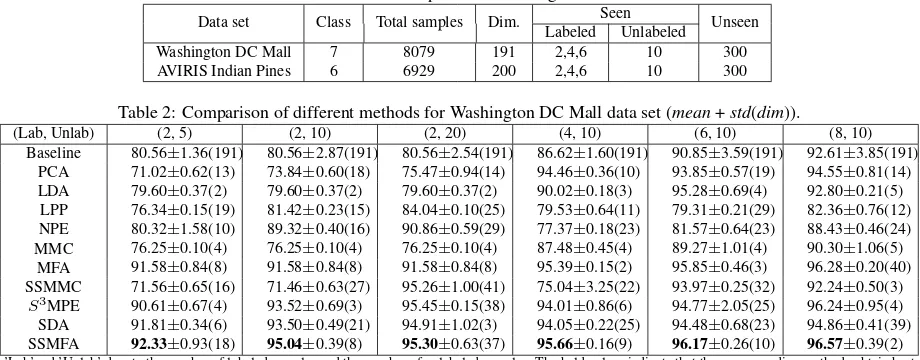
Table 1: Experimental settings.
Data set Class Total samples Dim. Seen Unseen
Labeled Unlabeled
Washington DC Mall 7 8079 191 2,4,6 10 300
AVIRIS Indian Pines 6 6929 200 2,4,6 10 300
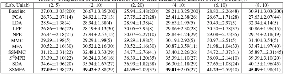
Table 2: Comparison of different methods for Washington DC Mall data set (mean+std(dim)).
(Lab, Unlab) (2, 5) (2, 10) (2, 20) (4, 10) (6, 10) (8, 10)
Baseline 80.56±1.36(191) 80.56±2.87(191) 80.56±2.54(191) 86.62±1.60(191) 90.85±3.59(191) 92.61±3.85(191) PCA 71.02±0.62(13) 73.84±0.60(18) 75.47±0.94(14) 94.46±0.36(10) 93.85±0.57(19) 94.55±0.81(14) LDA 79.60±0.37(2) 79.60±0.37(2) 79.60±0.37(2) 90.02±0.18(3) 95.28±0.69(4) 92.80±0.21(5)
LPP 76.34±0.15(19) 81.42±0.23(15) 84.04±0.10(25) 79.53±0.64(11) 79.31±0.21(29) 82.36±0.76(12) NPE 80.32±1.58(10) 89.32±0.40(16) 90.86±0.59(29) 77.37±0.18(23) 81.57±0.64(23) 88.43±0.46(24) MMC 76.25±0.10(4) 76.25±0.10(4) 76.25±0.10(4) 87.48±0.45(4) 89.27±1.01(4) 90.30±1.06(5)
MFA 91.58±0.84(8) 91.58±0.84(8) 91.58±0.84(8) 95.39±0.15(2) 95.85±0.46(3) 96.28±0.20(40) SSMMC 71.56±0.65(16) 71.46±0.63(27) 95.26±1.00(41) 75.04±3.25(22) 93.97±0.25(32) 92.24±0.50(3) S3MPE 90.61±0.67(4) 93.52±0.69(3) 95.45±0.15(38) 94.01±0.86(6) 94.77±2.05(25) 96.24±0.95(4)
SDA 91.81±0.34(6) 93.50±0.49(21) 94.91±1.02(3) 94.05±0.22(25) 94.48±0.68(23) 94.86±0.41(39) SSMFA 92.33±0.93(18) 95.04±0.39(8) 95.30±0.63(37) 95.66±0.16(9) 96.17±0.26(10) 96.57±0.39(2) ’Lab’and ’Unlab’ denote the number of labeled samples and the number of unlabeled samples. The bold values indicate that the corresponding methods obtain best
performances under specific conditions. And this notes for each table.
rates on different dimensions. Table 2 reports the best perfor-mance of different methods.
As can be seen from Table 2, for unsupervised and semi-supervised methods, the recognition accuracy increases with the increase in the extra sample size of the unlabeled set. Clearly, the semi-supervised methods outperform the semi-supervised counterparts, which indicates that combining the information provided by the labeled and unlabeled data gives the benefits to hyperspectral image clas-sification. In most cases, SSMFA outperforms all the other meth-ods.
To investigate the influence of the numbers of labeled data on the performances of semi-supervised algorithms, we replace the 2 la-beled data in semi-supervised algorithms with 4, 6 and 8 lala-beled data, respectively. As expected, the classification accuracy rises with the increase in the labeled sample size. Note that SSMMC and SSMFA don’t improve much on MMC and MFA when 8 la-beled data for training, because 8×7 = 56 labeled examples are quite enough to discriminate the data and therefore the effects of unlabeled data has been limited.
4.2.4 Experimental Results on AVIRIS Indian Pines Data Set In each experiment, we randomly select the seen and un-seen set according to Table 1, and the top 50 features were se-lected from AVIRIS Indian Pines data set by different methods. The results are shown in Table 3.
As can be seen from Table 3, all semi-supervised methods are all superior to supervised and unsupervised methods, which indi-cates that combining the information provided by the labeled and unlabeled data gives the benefits to feature selection for hyper-spectral image classification. Our SSMFA method also outper-forms the semi-supervised counterparts in most cases. Neverthe-less, for unsupervised and semi-supervised methods, the classi-fication accuracy increases with the increase in the extra sample size of the labeled set.
It’s obvious that the semi-supervised methods greatly outperform the other methods and that SSMFA performs better than oth-ers semi-supervised methods. Nevertheless, most methods don’t achieve good performance in this data set. One possible rea-son for the relatively poor performance of different methods in the data set lies in the strong mixture of the class signatures of AVIRIS Indian Pines data set. Hence, it is very interesting to de-velop more effective method to further improve the performance of hyperspectral image classification under complex conditions.
4.3 Discussion
The experiments on synthetic data and two hyperspectral image databases have revealed some interesting points.
(1) As more labeled data are used for training, the classification accuracy increases for all supervised and semi-supervised algo-rithms. This shows that a large number of labeled samples give benefits to identify the relevant features for classification.
(2) Semi-supervised methods, i.e. S3MPE, SDA and SSMFA, consistently outperform the supervised and unsupervised meth-ods, which indicates that semi-supervised methods can take ad-vantage of both labeled and unlabeled data points to find more discriminant information for hyperspectral image classification.
(3) An effective learning method can improve the performance when the number of the available unlabeled data increases. As expected, the recognition rate of the semi-supervised and unsu-pervised methods are significantly improved when the number of the available unlabeled data increases in Tables 2-3. Mean-while, the supervised methods, i.e. MMC and LDA, degrade the performance of classification accuracy due to the overfitting or overtraining.
(4) As shown in Tables 2-3, it is clear that SSMFA performs much better than other semi-supervised methods and MFA achieves a good performance than other supervised methods. This is due to that many methods, i. e. LDA and MMC, assume a Gaussian dis-tribution with the data of each class. MFA and SSMFA provide a proper way to overcome this limitations. Furthermore, SSMFA outperforms MFA in most cases. MFA can only use the labeled data, while SSMFA makes full use of the labeled and unlabeled data points to discover both discriminant and geometrical struc-ture of the data manifold.
5 CONCLUSIONS
The application of machine learning to pattern classification in the area of hyperspectral image is rapidly gaining interest in the community. It is a very challenging issue of urgent importance to select a minimal and effective subset from those mass of bands.
Table 3: Comparison of different methods for AVIRIS Indian Pines data set (mean+std(dim)).
(Lab, Unlab) (2, 5) (2, 10) (2, 20) (4, 10) (6, 10) (8, 10)
Baseline 27.00±3.03(200) 26.67±3.85(200) 25.94±2.48(200) 28.21±3.25(200) 28.80±2.26(48) 30.91±3.03(200) PCA 26.73±2.07(14) 24.92±1.72(13) 27.75±2.27(28) 25.41±2.38(26) 26.67±1.71(28) 27.63±2.07(44) LDA 28.94±1.38(4) 28.94±1.38(4) 28.94±1.38(4) 29.63±1.95(5) 30.49±2.97(5) 32.94±4.14(5)
LPP 26.86±1.96(22) 28.19±4.13(30) 30.05±3.95(8) 29.86±2.30(28) 30.50±1.78(37) 30.86±1.96(15) NPE 26.44±2.18(21) 27.94±2.57(15) 30.07±2.27(10) 28.84±1.24(29) 29.08±2.75(35) 29.74±2.18(19) MMC 29.29±1.98(5) 29.29±1.98(5) 29.29±1.98(5) 30.19±2.92(5) 30.97±2.51(5) 31.40±3.54(5)
MFA 30.52±2.16(30) 30.52±2.16(30) 30.52±2.16(30) 30.87±3.59(11) 31.98±1.04(33) 33.47±1.97(40) SSMMC 31.12±2.31(22) 32.48±3.33(29) 34.77±2.76(41) 33.40±2.26(26) 34.72±3.37(31) 35.897±2.31(45)
S3MPE 33.39±3.10(22) 36.24±3.36(16) 36.39±1.20(35) 35.39±1.10(27) 36.09±2.14(10) 39.39±3.10(20)
SDA 34.64±1.96(20) 35.54±1.67(27) 36.99±1.82(38) 36.30±1.18(29) 37.65±1.08(24) 40.15±1.96(45) SSMFA 37.09±1.98(22) 39.42±2.88(29) 41.95±2.09(37) 39.01±2.05(27) 41.23±2.59(40) 45.09±1.98(41)
two prominent characteristics. First, it is designed to achieve good discrimination ability by utilizing the labeled and unlabeled data points to discover both discriminant structure of the data manifold. In SSMFA, the labeled points are used to maximize the inter-manifold separability between data points from different classes, while the unlabeled points are used to minimize the intra-manifold compactness between data points belong to the same class or neighbors. Second, it provides a proper way to overcome the limitations that many dimensionality reduction methods as-sume a Gaussian distribution with the data of each class, which further improves hyperspectral image recognition performance. Experimental results on synthetic data and two well-known hy-perspectral image data sets demonstrate the effectiveness of the proposed SSMFA algorithm.
ACKNOWLEDGEMENTS
This work is supported by National Science Foundation of China (61101168), the Chongqing Natural Science Foundation (CSTC-2009BB2195), and the Key Science Projects of Chongqing Sci-ence and Technology Commission of China (CSTC2009AB2231). The authors would like to thank the anonymous reviewers for their constructive advice. The authors would also like to thank D. Landgrebe for providing the hyperspectral image data sets.
REFERENCES
S. J. Li, H. Wu, D. S. Wan, J. .l. Zhu, ”An effective feature selection method for hyperspectral image classification based on genetic algorithm and support vector machine,”Knowledge-Based Systems, vol. 24, no. 1, pp. 40-48, 2011.
I. Guyon, A. Elisseeff, ”An introduction to variable and feature selection,”
J. Machine Learning Research, vol. 3, pp. 1157-1182, 2003.
A. Plaza, J. A. Benediktsson, J. W. Boardman et al., ”Recent Advances in Techniques for Hyperspectral Image Processing,”Remote Sensing of Environment, vol. 113, no. 1, pp. 110-122, 2009.
H. Huang, J. W. Li, H. L. Feng, ”Subspaces versus submanifolds: a com-parative study in small sample size problem,”Int. J. Pattern Recognition and Artificial Intelligence, vol. 23, no. 3, pp. 463-490, 2009.
S. G. Chen and D. Q. Zhang, ”Semisupervised Dimensionality Reduction With Pairwise Constraints for Hyperspectral Image Classification,”IEEE Geoscience and Remote Sensing Letters, vol. 8, no. 2, pp. 369-373, Jan. 2011.
G. T. Kaya, O. K. Ersoy, and M. E. Kamas¸ak, ”Support Vector Selection and Adaptation for Remote Sensing Classification,”IEEE Trans. Geo-science and Remote Sensing, vol. 49, no. 6, pp. 2071-2079, June 2011.
H. Yang, Q. Du, H. J. Su, Y. H. Sheng, ”An Efficient Method for Su-pervised Hyperspectral Band Selection,”IEEE Geoscience and Remote Sensing Letters, vol. 8, no. 1, pp. 138-142, Jan. 2011.
B. Paskaleva, M. M. Hayat, Z. P. Wang, J. S. Tyo, and S. Krishna, ”Canon-ical Correlation Feature Selection for Sensors With Overlapping Bands: Theory and Application,”IEEE Trans. Geoscience and Remote Sensing, vol. 46, no. 10, pp. 3346-3358, October 2008.
H. Huang, J. M. Liu, H. L. Feng, T. D. He, ”Enhanced semi-supervised local Fisher discriminant analysis for face recognition,”Future Genera-tion Computer Systems, vol. 28, no. 1, pp. 244-253, 2011.
H. Huang, J. W. Li, J. M. Liu, ”Ear recognition based on uncorrelated local Fisher discriminant analysis,”Neurocomputing, vol. 74, no. 17, pp. 3103-3113, 2011.
S. T. Roweis,and L. K. Saul, ”Nonlinear Dimensionality reduction by locally linear embedding, Science,” vol.290, no. 5500, pp. 2323-2326, 2000.
J. B. Tenenbaum, V. de Silva, J. C. Langford, ”A global geometric frame-work for nonlinear dimensionality reduction,”Science, vol.290, no. 5500, pp. 2319-2323, 2000.
M. Belkin and P. Niyogi, ”Laplacian eigenmaps for dimensionality re-duction and data representation,”Neural Computation, vo. 15, no.6, pp. 1373-1396, 2003.
X. F. He, S. Yan, Y. Hu, et al, ”Face recognition using Laplacianfaces,”
IEEE Trans. Pattern Anal. Mach. Intell., vol.27, no. 3, pp. 328-340, 2005. X. F. He, D. Cai, and S. C. Yan, et al, ”Neighborhood preserving embed-ding,” in Proc. 10th Int. Conf. Computer Vision, 2005, pp. 1208-1213. D. Cai, X. F. He, and K. Zhou, ”Locality sensitive discriminant analysis,” in Proc. Int. Conf. Artificial Intelligence, Hyderabad, India, 2007, pp. 708-713.
S. Yan, D. Xu, B. Zhang, et al, ”Graph embedding and extensions: a general framework for dimensionality reduction,”IEEE Trans. Pattern Anal. Mach. Intell., vol. 29, no. 1, pp. 40-51, 2007.
G. Camps-Valls, T. Bandos Marsheva, D. Zhou, ”Semi-Supervised Graph-Based Hyperspectral Image Classification,” IEEE Trans. Geo-science and Remote Sensing, vol. 45, no. 10, pp. 3044-3054, 2007. S. Velasco-Forero and V. Manian, ”Improving hyperspectral image classi-fication using spatial preprocessing,”IEEE Geoscience and Remote Sens-ing Letters, vol. 6, no. 2, pp. 297-301, 2009.
D. Tuia and G. Camps-Valls, ”Semi-supervised Hyperspectral Image Classification with Cluster Kernels,”IEEE Geoscience and Remote Sens-ing Letters, vol. 6, no. 2, pp. 224-228, 2009.
Y. Q. Song, F. P. Nie, C.S. Zhang, S. M. Xiang, ’A unified framework for semi-supervised dimensionality reduction,”Pattern Recognition, vol. 41, no. 9, pp. 2789-2799, 2008.
X. J. Zhu and A. B. Goldberg, ”Introduction to Semi-Supervised Learn-ing,”Morgan & Claypool, 2009.
H. Y. Zha and Zh. Y. Zhang, ”Spectral Properties of the Alignment Ma-trices in Manifold Learning,”SIAM Review, vol. 51, no. 3, pp. 545-566, 2009.
H. Li, T. Jiang, and K. Zhang, ”Efficient and robust feature extraction by maximum margin criterion,”IEEE Trans. Neural Networks, vol. 17, no. 1, pp. 157-165, 2006.
Y. Q. Song, F. P. Nie, C. S. Zhang, S. M. Xiang, ”A unified framework for semi-supervised dimensionality reduction,”Pattern Recognition, vol. 41, no. 9, pp. 2789-2799, 2008.
Y. Q. Song, F. P. Nie, C. S. Zhang, ”Semi-supervised sub-manifold dis-criminant analysis,”Pattern Recognition, vol. 29, no. 13, pp. 1806-1813, 2008.
D. Cai, X. F. He, J. W. Han, ”Semi-Supervised Discriminant Analysis,” in Proc. the 11th IEEE International Conference on Computer Vision (ICCV07), Rio de Janeiro, Brazil, Oct. 2007.