GRAPH-BASED URBAN LAND USE MAPPING FROM HIGH RESOLUTION SATELLITE
IMAGES
I. Waldea,b, S. Hesea,b, C. Bergera, C. Schmulliusa,b
a
Friedrich-Schiller-University Jena, Institute of Geography, Earth Observation, bGraduate School on Image Processing and Image Interpretation (irene.walde, soeren.hese, christian.berger, c.schmullius)@uni-jena.de
Commission IV/3
KEY WORDS:Land Use, Land Cover, Urban, Modelling, Planning, High resolution, Structure, Value-added
ABSTRACT:
Due to the dynamic character of urban land use (e.g. urban sprawl) there is a demand for frequent updates for monitoring, modeling, and controlling purposes. Urban land use is an added value that can be indirectly derived with the help of various properties of land cover classes that describe a certain area and create a distinguishable structure. The goal of this project is to extract land use (LU) classes out of a structure of land cover (LC) classes from high resolution Quickbird data and additional LiDAR building height models. The study area is Rostock, a German city with more than 200.000 inhabitants. To model the properties of urban land use a graph based approach is adapted from other disciplines (industrial image processing, medicine, informatics). A graph consists of nodes and edges while nodes describe the land cover and edges define the relationship of neighboring objects. To calculate the adjacency that describes which nodes are combined with an edge several distance ranges and building height properties are tested. Furthermore the information value of planar versus non-planar graph types is analyzed. After creating the graphs specific indices are computed that evaluate how compact or connected the graphs are. In this work several graph indices are explained and applied to training areas. Results show that the distance of buildings and building height are reliable indicators for LU-categories. The separability of LU-classes improves when properties of land cover classes and graph indices are combined to a LU-signature.
KURZFASSUNG:
Aufgrund des dynamischen Charakters von St¨adten (Suburbanisierung/Zersiedelung) entsteht ein Bedarf an regelm¨aßiger Aktualisie-rung urbaner Landnutzungsdaten f¨ur ModellieAktualisie-rungs-, ¨Uberwachungs- und Kontrollzwecke. Urbane Landnutzung stellt einen Mehrwert dar, der mit Hilfe von spezifischen Eigenschaften von Landbedeckungsklassen, die ein bestimmtes Gebiet beschreiben und eine er-kennbare Struktur bilden, indirekt abgeleitet werden kann. Das Ziel des Projektes ist die Extraktion st¨adtischer Landnutzungstypen aus Landbedeckungsklassen, die aus hochaufgel¨osten optischen Quickbird-Satellitendaten und einem LiDAR-Oberfl¨achenmodell ab-geleitet wurden. Das Untersuchungsgebiet Rostock ist eine deutsche Stadt mit mehr als 200.000 Einwohnern. Um die Eigenschaften der Stadtstrukturen zu modellieren wurde ein graphenbasierter Ansatz, der bereits in anderen Wissenschaftszweigen (industrielle Bild-verarbeitung, Medizin, Informatik) eingesetzt wird, adaptiert. Ein Graph besteht aus Knoten, die die Landbedeckung repr¨asentieren, und Kanten, die die Eigenschaften zu benachbarten Objekten definieren. Um die Adjazenzmatrix zu berechnen, die beschreibt welche Knoten und Kanten miteinander verbunden sind, wurden verschiedene Distanzbereiche und H¨ohenangaben getestet. Dar¨uber hinaus wurde der Informationswert planarer und nicht-planarer Graphen analysiert. Nach der Graphenbildung wurden spezifische Indikato-ren berechnet, die beschreiben wie kompakt oder zusammenh¨angend der Graph ist. In diesem Paper werden einige dieser IndikatoIndikato-ren beschrieben und auf Trainingsgebiete angewandt. Die Ergebnisse zeigen, dass Geb¨audedistanzen und Geb¨audeh¨ohen zuverl¨assige In-dikatoren f¨ur bestimmte Landnutzungskategorien sind. Die Trennbarkeit urbaner Landnutzungstypen kann verbessert werden, indem man die Werte der Graphenindikatoren unterschiedlicher Strukturgraphen eines Gebietes zu einer Landnutzungssignatur verbindet.
1 INTRODUCTION
The UN Habitat announced in their annual report in 2010 that 52% of the global population is living in cities. By 2030 it is fore-casted that 60% of the world will be urban (UN Habitat, 2011). Urbanization is the least reversible human dominated LU-type. The consequences range from land cover change to climate im-pacts, habitat loss, or extinction of species. Additionally it influ-ences transportation developments, energy demand, or the auto-mobile market (Seto et al., 2011). The main drivers in Europe, mentioned by the European Environment Agency, are e.g. popu-lation increase, rising living standards and improvement of qual-ity of life, economic growth and globalization, policies and
distin-guish between a residential area, an industrial area, or a city core in high resolution satellite images. This is because the human per-ception works in a holistic way. The Gestalt-theory defines rules that describe how the human brain interprets complex structures. Proximity and similarity for example suggest patterns. Further-more we try to simplify complex objects into basic geometrical shapes. The capability of the human brain can handle many of the rules at the same time. The challenging part is the imple-mentation and combination of Gestalt rules and the emulation of the human brain for automated image interpretation. Antrop and Van Eetvelde (2000) analyzed landscape metrics in suburban ar-eas with regards to holistic characteristics. The aim of the project described in this paper is the extraction of urban LU-categories using holistic land cover properties for graph generation and anal-ysis. Graphs, containing nodes and edges, are an abstract concept of real world phenomena representing objects and their relation-ship among each other. Land cover objects (e.g. building, tree, impervious surface) define the nodes while the edges are the con-nection in relation to properties like distance, area or perimeter, building height, etc.. After the description of the study site and the available datasets the graph theory is introduced. Some graph indices that characterize the connectivity or complexity of the graph are defined followed by a description how the graphs in the study area are computed and analyzed. The results are discussed and the future work is suggested.
2 RELATED WORK
Medicine and informatics disciplines concerning image process-ing and interpretation have been dealprocess-ing with graph theory for structural analysis and classification approaches for a long time. Deuker et al (2009) described various graph metrics of complex networks relating to the application in human brain networks. Magnetoencephalography (MEG)-Images from human brains in a resting state and solving a memory exercise were analyzed. Different frequency interval networks were generated and global graph metrics were calculated (clustering coefficient, path length, small-worldness, assortativity, hierarchy, etc.) and divided into first and second order graph metrics. Gunduz, Yener, and Gul-tekin (2004) accomplished a classification of brain cancer cells (glioma) based on topological properties in the tissue image. The graphs were created using an exponential function of the Eu-clidean distance and the Waxman model. Diverse graph metrics and an artificial neural network (ANN) classification were per-formed resulting in the classes: healthy, cancerous, and inflamed. Graph based derivation of urban LU-types was established by Barnsley and Barr (1997). They developed the data model named XRAG (eXtended Relational Attribute Graph) which consists not only of nodes and edges but also of properties associated with the nodes (area, perimeter) and edges (distance, direction) as well as labeling of the land cover, grouping, and the probability of the assigned land cover class. The approach was based on raster data of a topographic map where land cover classes and their erties were derived. Morphological, relational, and spatial prop-erties were analyzed to distinguish between several urban areas with buildings from different decades. Bauer and Steinnocher (2001) used XRAG implemented in SAMS (Structural Analyzing and Mapping System) as a prerequisite for the definition of rules within eCognition software (Benz et al., 2004) to derive LU on a rule based method. De Almeida, Morley, and Dowman (2007) describe a graph based approach to analyze topological structures of urban regions. LiDAR data was triangulated and the slope of the resulting triangles was computed, followed by a classifica-tion of flat and steep polygons. Afterwards, depth-first search (DFS) and breadth-first search (BFS) algorithms were used to an-alyze how informative the graph-trees for the topological
prop-erty of containment are. Anders, Sester, and Fritsch (1999) pre-sented a graph clustering technique to infer higher level structures from detailed cadastral map data. A relative neighborhood graph (RNG) was computed by using a Delaunay Triangulation (DT) and outlier edges were removed. Furthermore the local neigh-bor density was calculated by using the size of the Voronoi cell around a node and the mean distance from the DT of linked nodes as an estimator.
3 STUDY SITE AND DATASET
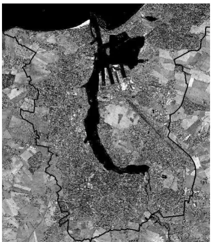
The study area is Rostock, a German Hanseatic city with more than 200.000 inhabitants built along the Warnow river until its embouchure in the Baltic Sea. A cloud-free 16-bit Quickbird satellite image with four channels (blue, green, red, and near-infrared) from September 2009 was used (Figure 1). After at-mospheric corrections a pan-sharpening of the multi-spectral im-age data was accomplished, resulting in a spatial resolution of 60 cm per pixel at the ground. LiDAR data from 2006 with a point density of two points per square meter was normalized with the digital elevation model to obtain the relative building and veg-etation heights (nDSM). Additional cadastral parcel and building polygons from January 2011 and an urban land use map, dig-itized from orthophotos from 2007, were beneficial for testing the methods on ideal training areas and will be helpful for the validation of the results . The Quickbird Ortho Ready Standard Imagery product did not include topographic correction and had a CE90 (Circular Error with 90% level of confidence) of 23 m or higher, depending on the terrain and the viewing angle (Cheng et al., 2003). For this reason a projective transformation with 30 well distributed ground control points from the cadastral building polygons and 3D information from the LiDAR elevation model was accomplished. In the first step ideal test areas for the differ-ent LU-classes were chosen. Therefore the essdiffer-ential land cover classes were combined from cadastral building polygons and a fusion of classes from the land use map and the nDSM. The fol-lowing land cover categories were derived: Built up, low built up, paved, trees, shrub, grass, water, and open land.
4 GRAPH THEORY
Graph theory is a branch of mathematics that had its initiation most likely in 1736 when Euler abstracted the problem of the ”Bridges of K¨onigsberg” into a simple graph and proved that a walk around K¨onigsberg crossing every bridge uniquely is impos-sible. It is an interdisciplinary science with various applications e.g. routing problems (shortest path algorithms, Traveling Sales-man problem), social and cognitive networks, technological net-works like the Internet, cell netnet-works or ecological netnet-works, in-frastructure networks, flow models, minimal costs computation, and many more. A graph consists of vertexes (nodes) and edges (links) (Caldarelli, 2007). A graph can be described with an ad-jacency matrix. The rows and columns of the adad-jacency matrix represent the vertexes while the entries denote if the vertexes are connected (1) or not (0). Graph indices represent structural prop-erties of graphs. The beta index (1) is a measure of connectivity and is computed by the ratio of edges (e) over vertexes (v) (Ro-drigue et al., 2009).
β=e
v (1)
The gamma index is a ratio of the observed edges over the number of maximum possible edges. Its value ranges between 0 and 1, where 1 represents a complete graph with no subgraphs. The formulas depend on the graph type. A planar graph (2) has no edge intersection outside of a vertex. In a non-planar graph (3) edge intersection must not result in a vertex followed by a higher number of possible links (Rodrigue et al., 2009, Stuttgart, 2011).
γ= e
3(v−2) (2)
γ= e
v(v−1) (3)
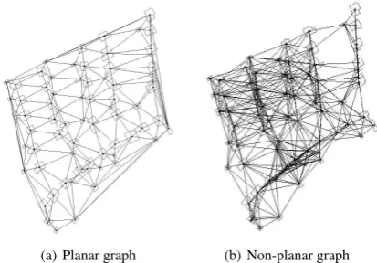
Figure 2 illustrate the difference between planar and non-planar graphs of a residential detached house area. The vertexes were generated from the centroids of the building polygons. The planar graph is the outcome of a Delaunay Triangulation.
(a) Planar graph (b) Non-planar graph
Figure 2: planar(a) and non-planar(b) graph of a residential de-tached house area
Another measure for connectivity is the alpha index which spec-ifies the redundancy of a net. It is defined as the number of cy-cles (meshes) over the maximum possible cycy-cles. The achieved values vary between 0 and 1, while 1 represents a completely connected graph. The formulas depend on the planar (5) and non-planar (6) graph type as well. A mesh is a chain where the start
and end node are the same and does not cross a link more than once. The number of cycles (u) (4) is estimated by a combination of nodes, links, and number of sub-graphs (p) which are subsets of a graph (Rodrigue et al., 2009, Stuttgart, 2011).
u=e−v+p (4)
α= u
2v−5 (5)
α= u
0.5∗(v(v−1))−(v−1)) (6)
More extensive graph measures that consider the internal com-plexity of a graph could reveal structural differences between net-works. The clustering coefficient, also referred to as transitivity in social network analysis, specifies if the neighbors of a vertex are also neighbors of each other. It unveils cluster or communities which have a similar degree of links. The clustering coefficient is divided into local and global, while the local clustering coefficient defines the clustering of a specific node, the global describes the clustering of the total graph. The local clustering coefficient (7) of a node is the proportion of edges of the vertexes in its neigh-borhood (ejk) by the maximum possible edges that could occur between them. Therefore the degree of the vertex (ki) is essen-tial, which indicates the number of outgoing edges or the number of adjacent nodes (Rodrigue, 2009).
Ci= 2
Pejk
ki(ki−1) (7)
The global clustering coefficient (8) indicates the overall proba-bility of a graph that neighboring nodes are connected. It is de-fined as the proportion of observed number of closed triplets over the maximum number of triplets. A triplet is a set of 3 nodes that is connected by two (open) or three (closed) edges (Rodrigue, 2009).
Ci=λG(v)
τG(v) (8)
The assortativity (9) is a coefficient of the Pearson correlation between node degrees. The derivation is well described in Cal-darelli (2007) or Newman (2002). It refers to the preference of a vertex to connect to vertexes of similar degree. The values range from -1 (disassortative graph) to 1 (assortative graph). In disas-sortative graphs nodes with very different degrees are connected and they often occur in strong hierarchical structures while social networks are typically assortative networks (Bassett et al., 2011, Deuker et al., 2009, Caldarelli, 2007, Rodrigue, 2009). The net-work assortativity function is stated as
r=
5 DATA ANALYSIS
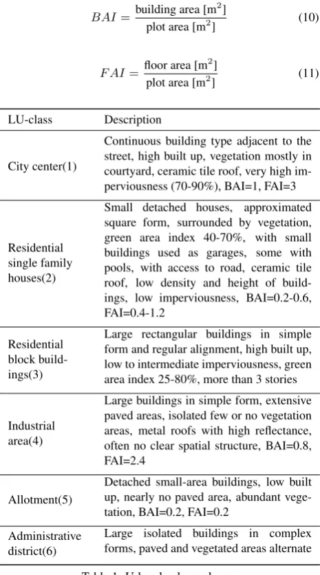
The first goal of the project was to define urban typology and to test the graph measures on significant training areas with the help of the properties of ideal cadastral and topographic data. Six meaningful urban LU-classes relevant for German urban fabric were established and listed in Table 1. Specific characteristics such as imperviousness or green area index were transfered from Banzhaf and H¨ofer (2008) . The German Federal Land Utiliza-tion Ordinance (Bundesministerium der Justiz, n.d.) constitutes the upper limit of the measure of the building area (10) and of the floor area (11). Both indices are allocated to the urban LU-classes in Table 1.
BAI=building area [m 2]
Continuous building type adjacent to the street, high built up, vegetation mostly in courtyard, ceramic tile roof, very high im-perviousness (70-90%), BAI=1, FAI=3
Residential single family houses(2)
Small detached houses, approximated square form, surrounded by vegetation, green area index 40-70%, with small buildings used as garages, some with pools, with access to road, ceramic tile roof, low density and height of build-ings, low imperviousness, BAI=0.2-0.6, FAI=0.4-1.2
Residential block build-ings(3)
Large rectangular buildings in simple form and regular alignment, high built up, low to intermediate imperviousness, green area index 25-80%, more than 3 stories
Industrial area(4)
Large buildings in simple form, extensive paved areas, isolated few or no vegetation areas, metal roofs with high reflectance, often no clear spatial structure, BAI=0.8, FAI=2.4
Allotment(5)
Detached small-area buildings, low built up, nearly no paved area, abundant vege-tation, BAI=0.2, FAI=0.2
Administrative district(6)
Large isolated buildings in complex forms, paved and vegetated areas alternate
Table 1: Urban land use classes
5.1 Analysis of planar and non-planar building graphs
To generate the graphs and compute the graph indices MatlabR
in combination with the additional Matgraph and the Brain Con-nectivity Toolbox were used. After importing the land cover poly-gons the centroids, representing the graph nodes, were computed to approximate the objects. To create planar graphs a Delaunay Triangulation of the building centroids was performed, which represents the spatial relationship between the building objects and can be referred to as relative neighborhood graph (RNG). Afterwards edges with a distance above 50 m were thinned out.
Non-planar graphs were generated with the help of the distance matrix containing all distances from one building node to all other building nodes. To compare the graph types edges above 50 m were deleted respectively. The graph indices were computed and the results are summarized in Table 2 and Table 3.
LU-class β γ(%) α(%) Clust.Coeff Assort.
1 2,84 94,86 92,28 0,39 −0,02
Table 2: Graph measures of planar building graphs
LU-class β γ(%) α(%) Clust.Coeff Assort.
1 12,84 1,83 3,39 0,62 0,70
Table 3: Graph measures of non-planar building graphs
The absent values for allotment areas resulted from lacking build-ing objects over 3 m in height. Comparbuild-ing graphs containbuild-ing low built up objects the allotment areas had high values of beta, gamma, and alpha indices while most of the other LU-classes had zero entries. Table 2 shows that the beta, gamma, and al-pha indices correlate with each other and that the city center had the highest values, representing the dense building structure. The lowest values were achieved by the industrial area. This indi-cates that the distance of 50 m is not sufficient for a well con-nected graph. Because of the low assortativity values the planar graphs of all LU-classes were neither assortative nor disassorta-tive. The administrative district had the highest clustering value for planar and non-planar graphs which denoted the occurrence of several communities. The gamma and alpha indices of non-planar graphs correlated while the beta index was not in line with the other two connectivity measures. Nevertheless, the ranking of the LU-classes regarding the values of the beta index was the same as with planar graphs. The values for assortativity increased immensely for non-planar graphs especially for the city center, which is a sign for an evenly distributed node degree and a ho-mogeneous structure.
5.2 Comparison of different distance ranges of planar build-ing graphs
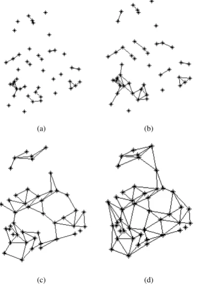
For the second approach planar building graphs were tested with different distance ranges. After a Delaunay Triangulation of the Centroids of the LU-training classes the distribution of the dis-tances of the edges were visualized in a box plot (Figure 3) to derive the distance ranges from the lower and upper quartile and the median. The overlapping distance ranges of 0-30 m, 10-40 m, 30-60 m, and 30-80 m were achieved to allow us investigate the separability. The edge outliers of the graphs were thinned out and the measures were computed. Looking at the different dis-tance ranges the graph structure changes. E.g. in the industrial area the graph changes from a sparsely connected in the 0-30 m range to a multiple connected graph in the 30-80 m range.
Figure 3: Edge distances after Delaunay Triangulation
(a) (b)
(c) (d)
Figure 4: Planar graphs of industrial area: (a) distance range 0-30 m; (b) 10-40 m; (c) 0-30-60 m; and (d) 0-30-80 m.
5.3 Using graph based measures for creating a LU-signature
Because beta, gamma, and alpha index correlate in planar graphs just the beta index was discussed. Furthermore the idea of a beta index-based LU-signature was introduced. In Figure 5 the beta index of the LU-training areas for the 4 distance ranges was pre-sented. Administrative district, city center, and residential single family houses started with a higher beta index and showed a de-cline in the classes with the broader distances. The beta index of the industrial area and residential block buildings showed the op-posite behavior and rose with broader distances. A straight line combines the values to distinguish the separability. The approach for the future work is to develop a land use signature for several graph measures and to assign the LU-classes on the basis of their membership to a specific signature.
Also the assortativity showed significant changes passing the
dis-Figure 5: Beta index of planar graphs for different distance ranges
tance ranges. Residential single family houses and residential block building graphs appeared to have assortative behavior in the lower distant range (Figure 6).
Figure 6: Assortativity of planar graphs for different distance ranges
5.4 Significance of different roof types of planar building graphs
Because there is potential to classify different roof types based on reflectance values in high resolution satellite images the graphs were investigated concerning red and dark ceramic roof tiles. Pla-nar graphs with an edge distance of 0 to 50 m were examined and the results of the beta index were summarized in Table 4.
LU-class red roof dark roof
City center 2,34 2,83
Residential single family houses 1,73 2,22
Residential block buildings 1,95 1,33
Industrial area 0 1,65
Administrative district 0 2,07
Table 4: Beta index of different roof type graphs
6 CONCLUSION AND FUTURE WORK
The introduced graph measures applied on ideal training areas showed potential for land use class extraction. The beta index of planar and non-planar graphs identified the city center as the densest structure while the clustering coefficient showed the high-est values for the administrative district. Beta, gamma, and al-pha index correlated in planar graphs. In contrast to non-planar graphs where gamma and alpha index correlated, the beta index did not correlate. The assortativity values for non-planar graphs increased compared to those from planar graphs. The city center appeared as an assortative graph which was an indicator for an evenly distributed node degree and hence a homogeneous struc-ture. The beta index signature of distance range-graphs was a sig-nificant characteristic showing the development of graphs accord-ing to the edge attribute of distance. Saccord-ingle family houses and the city center showed a decrease of the beta index with broader distances while industrial areas and residential block buildings have the opposite properties. The significance of red and dark roof types was investigated revealing that all residential urban LU-classes (single family buildings, block buildings, city cen-ter) had similar densities for red and dark roofs. Industrial areas and administrative areas had a denser structure of dark roofs and an empty graph (no edges) for red roofs (denoting the absence or isolated occurrence). A study with metallic (bright) roofs should be performed assuming a frequent appearance in industrial areas. Further research has to be done concerning graphs with several node (land cover type, area, compactness, etc.) and edge (dis-tances, orientation, weights, etc.) attributes. The indices have to be applied on a set of reference areas as well as on derived land cover datasets from high resolution satellite images. Additional to the distance as a spatial attribute also the building heights, ar-eas, and direct neighborhood will be analyzed. Allotment areas are well distinguished with respect to the building height as a rel-ative characteristic for graph generation. The green area index, imperviousness, building area as well as floor area index as indi-cated in the urban land use definitions should be converted into graph structure characteristics. The mentioned land use signature has to be developed further based on the combination of various graph properties in order to achieve a better LU-class separabil-ity. The adoption of supervised machine learning methods will be utilized to analyze various graphs and graph measures simul-taneously.
ACKNOWLEDGEMENTS
Very much acknowledged is the financial support of the ProExzel-lenz initiative of the ”Th¨uringer Ministerium f¨ur Bildung, Wis-senschaft und Kultur” (TMBWK), grant no. PE309-2. The au-thors are grateful to the land registry office of Rostock for the provision of the ALK, DLM, and LiDAR data. We greatly appre-ciate the thorough review and valuable comments of the anony-mous reviewers that helped to improve this paper.
REFERENCES
Anders, K.-H., Sester, M. and Fritsch, D., 1999. Analysis of set-tlement structures by graph-based clustering. Semantische Mod-ellierung, SMATI 99 pp. 41–49.
Antrop, M. and Van Eetvelde, V., 2000. Holistic aspects of sub-urban landscapes: visual image interpretation and landscape met-rics. Landscape and Urban Planning (50), pp. 43–58.
Banzhaf, E. and H¨ofer, R., 2008. Monitoring urban structure types as spatial indicators with cir aerial photographs for a more
effective urban environmental management. IEEE Journal of se-lected topics in Applied Earth Observations & Remote Sensing (Vol. 1, No. 2), pp. 129–138.
Barnsley, M. and Barr, S., 1997. Distinguishing urban land-use categories in fine spatial resolution land-cover data using a graph-based, structural pattern recognition system. Computers, Envi-ronment and Urban Systems Volume 21, Issues 3-4, pp. 209–225.
Bassett, D. S., Brown, J. A., Deshpande, V., Carlson, J. M. and Grafton, S. T., 2011. Conserved and variable architecture of hu-man white matter connectivity. NeuroImage 54(2), pp. 1262– 1279.
Bauer, T. and Steinnocher, K., 2001. Per-parcel land use clas-sification in urban areas applying a rule-based technique. Geo-BIT/GIS (6), pp. 24–27.
Benz, U. C., Hofmann, P., Willhauck, G., Lingenfelder, I. and Markus, H., 2004. Multi-resolution, object-oriented fuzzy analy-sis of remote sensing data for gis-ready information. ISPRS Jour-nal of Photogrammetry & Remote Sensing 2004(58), pp. 239– 258.
Bundesministerium der Justiz, n.d. Verordnung ¨uber die bauliche Nutzung der Grundst¨ucke (Baunutzungsverodnung - BauNVO): BauNVO.
Caldarelli, G., 2007. Scale-free networks: Complex webs in na-ture and technology. Oxford University Press, Oxford.
Cheng, P., Toutin, T., Zhang, Y. and Wood, M., 2003. Quickbird – geometric correction, path and block processing and data fusion. Earth Observation Magazine (vol. 12, no. 3), pp. 24–28.
De Almeida, J.-P., Morley, J. G. and Dowman, I. J., 2007. Graph theory in higher order topological analysis of urban scenes. Com-puters, Environment and Urban Systems 31(4), pp. 426–440.
Deuker, L., Bullmore, E. T., Smith, M., Christensen, S., Nathan, P. J., Rockstroh, B. and Bassett, D. S., 2009. Reproducibility of graph metrics of human brain functional networks. NeuroImage 47(4), pp. 1460–1468.
Di Gregorio, A., 2005. Land cover classification system software version 2: Based on the orig. software version 1. Environment and natural resources series Geo-spatial data and information, Vol. 8, rev. edn, Rome.
European Environment Agency, 2010. The european environ-ment: State and outlook 2010 - Land Use.
Gunduz, C., Yener, B. and Gultekin, S. H., 2004. The cell graphs of cancer. Bioinformatics 20(Suppl 1), pp. i145–i151.
Newman, M., 2002. Assortative mixing in networks. Physical Review Letters.
Rodrigue, J.-P., 2009. The geography of transport systems, http://people.hofstra.edu/geotrans (15.01.2012).
Rodrigue, J.-P., Comtois, C. and Slack, B., 2009. The geography of transport systems. 2 edn, Routledge, London.
Seto, K. C., Fragkias, M., G¨uneralp, B., Reilly, M. K. and A˜nel, J. A., 2011. A meta-analysis of global urban land expansion. PLoS ONE 6(8), pp. e23777.
Stuttgart, University, 2011.
Netzw-erke und Graphentheorie, http://www.ifp.uni- stuttgart.de/lehre/vorlesungen/GIS1/Lernmodule/Netzwerk-analyse/Graphentheorie/ (15.01.2012).