A Two-dimensional Model for the Transmission of
Dengue Fever Disease
*Edy Soewono1) & Asep K. Supriatna2) 1) Department of Mathematics & Center of Mathematics
Institut Teknologi Bandung Ganesha 10, Bandung 40132 2) Department of Mathematics
Universitas Padjadjaran Km 21 Jatinangor, Bandung 45363
INDONESIA
A transmission model for dengue fever is discussed here. Restricting the dynamics for the
constant host and vector populations, the model is reduced to a two-dimensional planar
equation. In this model the endemic state is stable if the basic reproductive number of the
disease is greater than one. A trapping region containing the heteroclinic orbit connecting the
origin (as a saddle point) and the endemic fixed point occurs. By the use of the heteroclinic
orbit, we estimate the time needed for an initial condition to reach a certain number of
infectives. This estimate is shown to agree with the numerical results computed directly from
the dynamics of the populations.
1. Introduction
Dengue fever is regarded as a serious infectious disease that risks about 2.5
billion people all over the world, especially in the tropical countries [2]. Mortality rate of
this infectious disease may reach 40 % if the infected person is left untreated [3].
Although almost all of the occurrences of the dengue are in the tropical countries, a
recent study shows that the dengue may occur in cooler countries due to the global
warming effects [4]. The climate change may convert a region from an unsuitable habitat
for Aedes aegypti mosquitoes to live to a new suitable habitat; the Aedes are the
responsible vector in transmitting the disease.
*
To control the dengue effectively, we should understand the dynamics of the
disease transmission and take into account all of the relevant details, such as the
dynamics of the vector. Recently Esteva and Vargas [1] developed a model for the
dengue disease transmission and included the dynamics of the Aedes aegypti mosquitoes
into a standard SIR (susceptible-infective-recover) epidemic model of a single
population. Their model shows that there is a threshold value R which is a function of
Aedes equilibrium population size and of the Aedes recruitment rate, above which the
disease will be endemic and below which the disease will vanish.
In developing their model, Esteva and Vargas assume that once a person recover
from the disease he or she will not re-infected by the disease. We show in this paper that,
in their model, if the Aedes recruitment rate is very large then only a small proportion of
the population becomes infected. This situation is not alarming and may not have a good
psychological effect on the management of the disease, that is, it may not persuade a
health manager to take a quick response in controlling the disease. In this paper we
remove the immunity assumption and predict the time needed by an initial number of
infected population to multiply. The result can alert us because for a large Aedes
recruitment rate, the time to multiply (e.g. ten times) is very short. In the next section we
review the model of Esteva and Vargas in more detail.
2. Host-Vector Model for a Dengue Transmission
We review the Host-Vector model of Esteva-Vargas [1] for the transmission of
dengue fever as follows. The model is based on the assumption that the host population
NH is constant, i.e. the death rate and birth rate are equal to μH. The vector population
, which is in general very difficult to estimate, is governed by a monotonic model
V
N
.
'
V V
V A N
N = −μ (1)
Here μN is the mortality rate of the vector, and A is the recruitment rate. This mosquito model can be explained from the fact that only a small portion of a large supply of eggs
survive to the adult stage [6]. Hence, A is independent from the adult population. The
In the Esteva-Vargas model [1] the majority of the host population eventually
becomes immune. The host population is subdivided into the susceptible , the
infective and the recovered, assumed immune, . The vector population, due to a
short life period, is subdivided into the susceptible and the infective .
H
The interaction model for the dengue transmission [1] is given as follows
Note that we remove the alternative blood resource from [1] due to the fact that
Further reduction of (2) to a three-dimensional dynamics is obtained from a
restriction to an invariant subset defined by
and .
The resulting dynamics, expressed in proportions
V
system are
(5)
Note that the second fixed point exists in the region of biological interest, i.e.
, only if the threshold parameter
1
R0 = represents the basic reproductive number. The following theorem has been proven in [1].
Theorem 1 If R≤1, the fixed point F1 is globally asymptotically stable in the region of
interest Ω={(x,y,z):0<x,y,z<1} and if R>1, F1 is unstable and the endemic fixed
Global stability of F1 forR<1 is shown in [1] using Lyapunov-like function z+ y
δ α
satisfying
0 ) 1 (
1 − − − <
⎟⎟⎠ ⎞ ⎜⎜⎝
⎛ − = ⎟ ⎠ ⎞ ⎜
⎝
⎛ z+ y y yz z x
dt d
α δ
αγ β δβ αγ δ
α
if R<1. On the other hand, if R>1 the fixed point F1 becomes locally unstable and F2
becomes locally asymptotically stable. The global stability is shown in [1] by use of the
property of stability of periodic orbits.
Note that α is the only parameter in (4) containing A. Study [4] has indicated that the mosquito population (and therefore the recruitment number A) may change from time
to time due to climate change. Although there is a report indicated that the biting
behavior of the mosquito has gradually changed and b is thought to vary with climate, we
assume that during a long period of observation, the biting rate b and the rest of the
parameters remain constant.
Regarding the control strategy for the epidemic, it is always the interest of
everyone to lower the basic reproductive number as small as possible (or equivalently
to lower the recruitment number A as small as possible). Various applications of
insecticides such as ULV have been used. Simulation of the application of ULV is shown
in [1]. It shows that the delay of the abrupt change of μ 0 R
V due to ULV will give effect to the delay of the endemic stage but will only slightly reduce the severity. The strategy to
lower R0 seems unrealistic as indicated by the reappearance of the outbreak almost every
year in the last 10 years. On the other hand, what is going to happen if A is so large? This
can be seen by taking the limit as A→∞. In this case, the endemic state approaches the
limit
. 1 , ,
0 2
⎟⎟⎠ ⎞ ⎜⎜⎝
⎛
+ →
H H
H
F
μ
γ μ (6)
It shows that although all mosquitoes are infected, only a small proportion of the human
population becomes infected, that is, H
H H
I μ γ
μ
γ μ+ <<
≈ H
H
since in this model the majority of the population eventually become immune (we will
remove the immunity condition in Section 3).
We are interested to investigate what happens if few infectives
(
)
areintroduced to the population. This illustrates, more or less, how the outbreak started. The
following pictures show the dynamics of the and in 100 days after one
infected human entered the population (all parameter values are taken from [1]). or V H I
I
H H I
S , IV
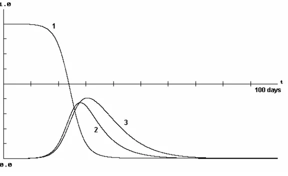
Figure 1: Dynamics of in 100 days with the initial condition
(0.9,0.0001,0) for
) 3 ( and (2) ), 1
( H V
H I I
S
, / 0000457
. day
H =
μ μV =.25/day,b=.5,βH =.75,βV =1, ,
/ 1428
. day
H =
γ NH =10,000 and A=5,000. With these parameters, R=3.24.
Figure 1 shows that drops significantly in a relatively small period of time. Both
and increases significantly during the period of 30 days, and then eventually oscillate
around the endemic state (0.09529,0.0.00029,0.00058). This seems unrealistic in the
nature. With constant population of mosquitoes, this fluctuation (in a short period of
time) can not be shown to happen in the nature. The sharp decrease of S
H
S IH
V
I
H and increase of
RH in the model (2) are due to the fact that μHRH is relatively smaller than both IHIV and SHIV at least in the domain of observation where IH in reality is relatively very small. The
3. Host-Vector Model without Immunity
Not enough information is known about the immunity after recovery. Reports
indicate that recovery from a certain serotype virus is not immune from other serotype
viruses (Dr. R. Agoes, MPH. Personal. Comm.). Assuming that immune subpopulation is
negligible, then we have the dynamics
(
)
Reducing the dynamics along invariant subsets
V
using the same notation for the proportion variables x and y as before, we have
( )
3.1 Stability of the endemic state
The corresponding characteristic equation of the fixed point (0,0) is
(
)
0.(this is equivalent to R>1), the origin becomes unstable and the second fixed point
, where second fixed point is
where a0 =α(δ(+γγ+δ) (2)(+γα+αβ+)β)2 . Both eigenvalues of (10) have negative real parts if R>1. Hence the second fixed point is locally stable. Global stability can be easily shown by
simple phase plane analysis with the direction of the vector fields of the system, as
indicated by the following theorem.
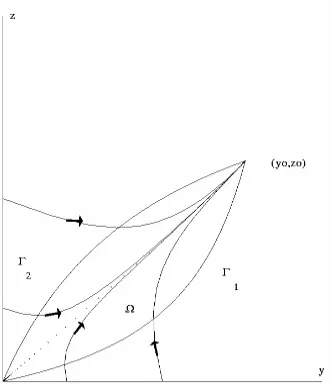
Theorem 2 Let Ω=
{
( )
y,z |α( )β1−yy ≤ z≤γyγ+yδ ,0≤ y≤ y0}
. If αγ −βδ >0, then is a trapping region and contains the heteroclinic orbit connectingΩ
( )
0,0 and(
x0, y0)
.Proof:
We write ∂Ω=Γ1∪Γ2, where Γ1 =
{
( ) ( ) ( )
y,z |G1 y,z ≡α 1−y z−βy =0,0< y< y0}
and( ) ( ) ( )
{
2 0}
2 = x,y |G x,y ≡ 1−z y− z=0, 0< y< y
Γ γ δ . Then along Γ1 and Γ2 we have
, 0 >
j dt
d
G j = 1,2. This shows that any orbit crossing ∂Ω is trapped inside Ω since the
gradient of along is pointing inward. With the vector field inside pointing
away from the origin we have the unstable manifold of the fixed point (0,0) connecting
the origin with the second fixed point. By rewriting
j
G ∂Ω Ω
1
Γ and Γ2in the form
) )( )( 1 (
) (
: 0
0 0 1
β α δ γ
αγ − −+ + +
= Γ
y y y y y
y z z
and
) )( )(
(
) (
: 0
0 0 2
β α δ γ δ γ
αγ +γ −+ + −
= Γ
y y y y y
y z
z ,
it can be seen that both Γ1 and Γ2 approach the line y y z z
0 0
Figure 2: Trapping region Ω. The dotted curve is the heteroclinic orbit
Further we will answer the question “how long it takes from a given initial
condition (one infective) to reach a certain stage ?”. In the neighborhood of (0,0), the
orbits quickly enter Ω and then follow close to the unstable manifold (the heteroclinic
orbit). Since the heteroclinic orbit is monotonic then it is reasonable to approximate this
orbit by a line connecting (0,0) and (x0,y0). Let the initial condition be
(
, theestimate time T to reach the infective can be done by integrating (8) along the line
)
0 , 0 y
1 y
y z yz
0 0
= as follow
( )
11
0
0 0
∫
− −= y y
y z
y y y
dy T
β α
(
) (
)
(
) (
)
. (11) lnln
0 1 0
1
⎭ ⎬ ⎫ ⎩
⎨ ⎧
− −
+ − −
+ −
−+ =
βδ αγ β α
γγ α β αγ βδ βδ
αγγ δ y
y y
y
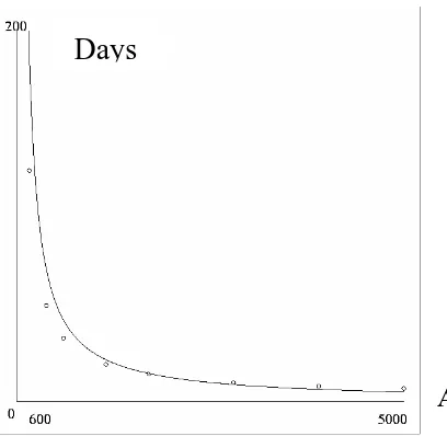
Note that as expected. Figure 3 shows comparison between (11) and
numerical calculation with PHASER [5]. It shows that it takes 186 days and 5 days for
one infective human to become 10 for 0
1
as
y y
T →∞ →
5000
and
600 =
= A
Days
A
Figure 3: Estimate time (days) needed from one infected human to become ten
(continuous graph) and the numerical calculation with PHASER directly from the dynamics in equation (8) (dotted graph).
4. Conclusion
We have shown the analysis of a two-dimensional dynamics of human-mosquito
interaction based on the host-vector model of Esteva-Vargas [1]. In the case of large
recruitment rate and when the number of infected human and infected vector are initially
very small, the trajectory quickly enters the trapping region, monotonically increases and
approaches the stable endemic state. Assuming that the fluctuation of the dynamics of
and is due to the change of the vector population, this ‘’monotonic’’ model is a good
representation for a short period simulation of the real situation. A study [7] has indicated
that the mosquito population, and therefore the recruitment number A, may change from
time to time due to climate changes. We discuss elsewhere the effects of a periodic
mosquito recruitment rate on the dengue transmission [8]. Further development of the
model can then be generated from the present model by adding relevant complexities,
such as human migration and vector dispersal.
H
I
V
Acknowledgement
We thank an anonymous referee who gave some valuable comments and suggestions in
improving the paper into the present form.
References
[1] L. Esteva, C. Vargas: Analysis of a dengue disease transmission model, Math.
Biosciences 150 (1998), 131-151.
[2] D.J. Gubler and G.C. Clark: Dengue/dengue hemorrhagic fever: the emergence of a
global health problem, Emerging Infectious Diseases 1 (1995), 55-57.
[3] A.S. Beneson: Control of communicable diseases in man, American Public Health
Association (1990), Washington D.C.
[4] J.A. Patz, P.R. Epstein, T.A. Burke and J.M. Balbus: Global climate change and
emerging infectious diseases, JAMA 275 (1996), 217-223.
[5] H. Kocak: Differential and difference equation through computer experiments,
Springer-Verlag (1980), NewYork.
[6] Dengue update. Proceeding. Universitas Padjadjaran (1992).
[7] L.M. Ruerda, K.J. Patel, R.C. Axtell and R.E. Stinner: Temperature-dependent
development and survival rates of Culex quiquefasciatus and Aedes aegypti (Diptera:
Culicidae). J. Med. Entomol. 27 (1990), 892-898.
[8] A.K. Supriatna and E. Soewono: A Mathematical model for the transmission of the